Does A Stock's Premium Make Sense: Analyzing Value Gain Functions

Originally published on: Does A Stock’s Premium Make Sense: Analyzing Value Gain Functions

If you ever found yourself analyzing an overvalued stock, only to return to it a year later and find it holding the same forecasts (t+1) but trading around intrinsic value, then you may be dealing with an accelerated value gain function.

The takeaway from this exploration is that investors can be more comfortable with higher premiums as quality companies may be able to converge on the fundamentals faster than anticipated, but should still react appropriately to narrative violations that change the forecast structure, as these can amplify value changes in both directions.

In other words, the future value gain function is more important for a company’s price than its present value. Some companies have linear value gain functions, but others – typically high growth along with excess ROIC, can have exponential value gain functions. These companies tend to be “value investor short traps”, as investors look at the price difference to the present value, assume linear value gain, and conclude that there is opportunity for going short on the stock.

Further, the notion that the IRR decreases as stocks become more expensive may be somewhat misleading, as the risk profile of a stock doesn’t necessarily change all that much when getting an influx of cheap equity financing, so lowering the IRR gain over the years may be misallocating the risk structure of an excess value stock to one of linear value. In other words, you aren’t dealing with a 2% IRR company, but one that will create value faster than its cost of capital. The 2% IRR breaks down the moment you advance 1 year, but you have screened yourself out of the investment.

For reference, a linear value stock is one that has its projected ROIC be roughly equal to the projected cost of capital, that is, ROIC = WACC. But an excess value stock is one where the projected ROIC > WACC. This poses the question “is penciling-out lower IRR values to these stocks the right approach?”

Let’s take a step back, I will divide the value gain function of stocks into 3 categories:

• Mature companies with stable growth: linear value gain function

• Stable growth, with high ROIC: linear value gain + excess value function

• High growth, high ROIC: exponential value gain using a rolling DCF

In my view, the reason we don’t tend to see many rolling DCF models is because they are hard to model in Excel and would require 10 valuation tables to get the final output, but we might be able to make them in code.

We can apply a single stage DCF model to these, and find that the value gain is roughly equal to the cost of capital. An 8% WACC stock will increase in value by the same amount less the dividend yield next year. In effect the Forward Value or Price Target for this stock becomes:

Forward Value = Intrinsic value * (1 + WACC) = 100 * (1 + 0.08) = 108

Note, for price appreciation (target), we need to subtract any cash dividends, so our price target becomes: Intrinsic value * (1 + WACC - Div. Yld), for example 100 * (1 + 0.08 - 0.03) = 105

While some analysts deem a single stage model to be beneath them as it implies a lack of alpha, this is likely the appropriate case for a larger majority of companies, excluding the ones in high and non-linear productive growth, or conversely the ones in decline.

We should also note the compounding effect as each passing year increases the value base, even though the value gain is fixed at the WACC. So you would project something like 100 * 1.08^3 in order to get the price target for year 3 of your model. That becomes 100 * 1.26 = 126, instead of 8 * 3 + 100, which would be 124. That 2-point difference is our compounding effect, which obviously gets larger with longer horizons.

Essentially, the single stage DCF is an inverted multiple, where you take the 1/PE(fwd), or appropriate bottom line multiple, and compare it to (r - g), that is, the WACC - growth.

So you may get something like 1/25 = 0.04, and divide it by its (r - g), for example 8% - 3%, resulting in (0.05/0.04 - 1) = 0.25 to find that the stock is 25% overvalued. Investors that have been used to high-growth, low interest environments, suddenly find themselves in deep water with a setup like this, because the notion that something trading at a forward multiple of 25x “is cheap” falls apart.

Conversely, TTM multiples are backwards looking and don’t tell you much other than a price stability reference, because the value of the stock is tied to its bottom line next year.

The second category are companies that tend to have growth rates in-line with the riskfree rate, and are disproportionately increasing their bottom line as they grow. Essentially, the way excess value shows up is by increasing the bottom line faster than the top line. While revenue growth may be 4%, free cash flows to equity may grow 10%, that 6% difference is the result of our higher ROIC.

Here, we have an asymmetric R/R (risk to reward) scenario where we have to calculate the value gain that is above the cost of capital. A caveat is that ROIC is rarely extraordinary, especially in stable growth companies, but we can save ourselves the trouble of non-linear ROIC by not modeling projections of forward value for more than 5, but ideally 2 years.

In order to incorporate the higher ROIC in our value gain we need to multiply it by the simple value gain. We build on the single-stage value gain function we had previously:

Intrinsic Value * [ROIC * ((WACC - Div. Yld) / WACC) +1]^years

Note: subtract the dividend yield from WACC to get the reinvestment rate.

So in our case, the forward value in year 1 comes up to:

100 * [0.1 * ((0.08 - 0.04) / 0.08) + 1] = 100 * (0.1 * 0.5 + 1) = 100 * 1.05 = 105

Or if the company does not pay dividends:

100 * (0.1 + 1) = 110

The difference between a stock that grows in-line with WACC and one that has an excess value is 108 vs. 110. In year 3 that difference comes up to 126 vs 133.1, a 5.6% difference.

Now, the forward value becomes:

• Intrinsic Value = 100

• Year 1 = 100 * 1.1 = 110, YoY delta = 10

• Year 2 = 100 * 1.1^2 = 100 * 1.21 = 121, YoY delta = 11, growth = 10%

• Year 3 = 100 * 1.1^3 = 100 * 1.331 = 133.1, YoY delta = 12.1, growth = 10%

• Year 4 = 100 * 1.1^4 = 100 * 1.461 = 146.41, YoY delta = 13.31, growth = 10%

The linear excess value gives us a 10% total value gain each year.

What if we have a 35% ROIC company instead of our 10% ROIC one?

Well, first off, if we have this scenario, we should check if the ROIC really is 35% by going through the financial statements and reasonably capitalizing R&D and marketing expenses. “Reasonably” means that we have to employ judgement on the weight of the capitalization, for example in a high tech company we would capitalize 100% of R&D, while in an acquisition compounder we may want to drop that to 40% and expense the rest. Second, high ROIC is unlikely and becomes unstable the higher it goes, the reason we see it so much is because investors typically focus on companies at the tip of the S&P 500. In this case we will have to treat the ROIC as non-linear and can’t employ a clean exponent, but would have to start by calculating the value gain for each year with a different ROIC weight. In this scenario, it is also likely that we have to incorporate an increasing number of moving parts (like non-linear growth), so analysts reach for a pull-forward DCF, but this is also lacking and we will explore why in the next part.

Imagine you are valuing Microsoft (MSFT) in 2016, you set your forecasts and a terminal value in 2026, year 10. You were bullish on Satya and somehow got the ballpark forecasts right. However, MSFT didn’t enter a terminal growth phase despite the age, and if you valued it as such you would have underestimated by how much the stock would have grown, more importantly, how much it would be worth today.

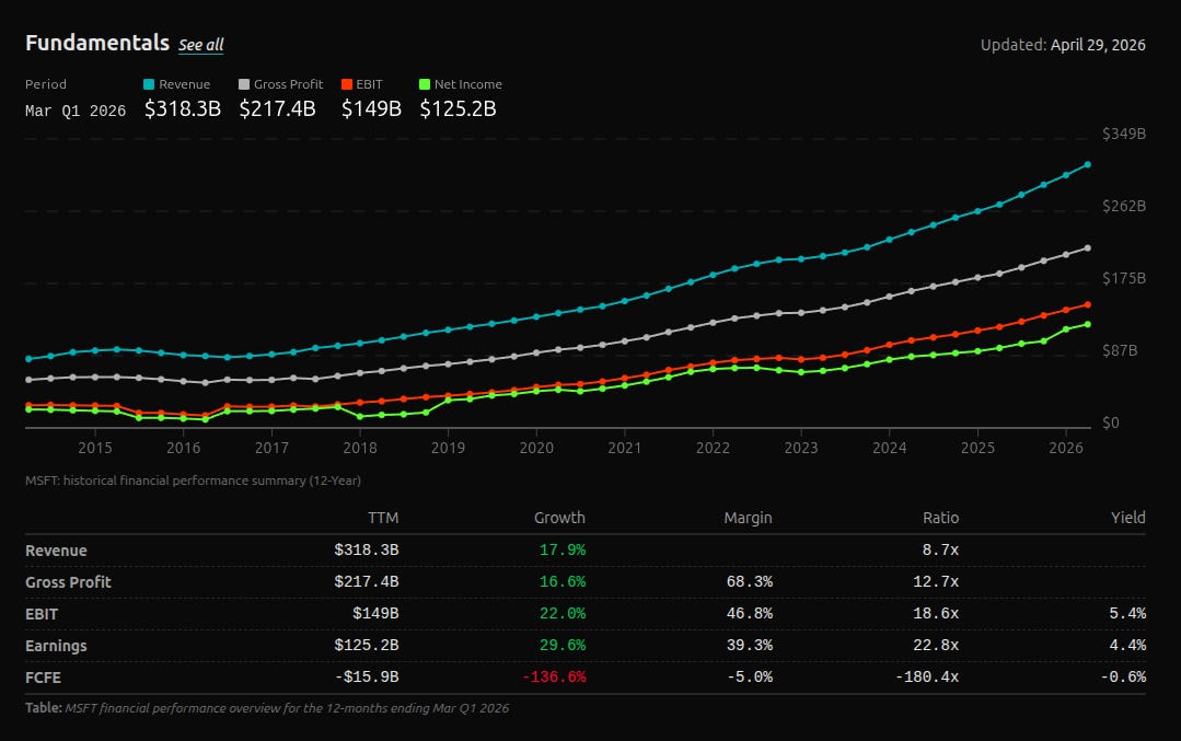
You could do a pull-forward valuation, and see the value of the company in the terminal year by using FCFEt / (r-g) and work back to see how much value would appreciate every year. But here is the problem with the pull-forward method: you are assuming that growth slows and stays around the riskfree rate. For many companies this is a reasonable assumption, but not for something like MSFT, which has been operating at a higher growth level for decades.

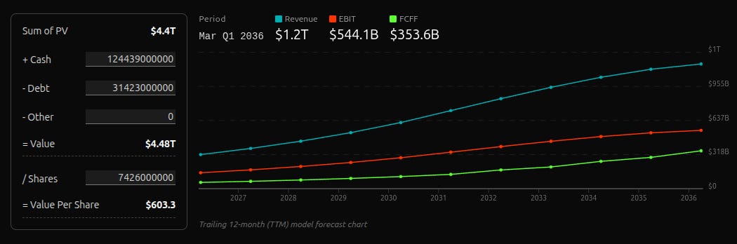
In this scenario you have at least 2 options:

• Use a long DCF model: 30-year+, and pull forward the valuation in year 30.

or

• Use a rolling DCF, and append a quarter every time the company publishes new results.

The rolling DCF and pull-forward DCFs strive to answer the same question: What is going to be the present value of an asset at each forecast year?

In my view, the rolling DCF approach is much easier to forecast as it requires maintaining a shorter decay function, making growth reacceleration easier to model. Your goal is not to be precise on the forecasts, even 10 years of forecasting is close to absurd, but your goal is to capture the shape of the value gain function.

There are a few factors that will contribute to this shape: growth cycles, incremental increases in profitability, reinvestment rates, idiosyncratic risk. Because the rate of change of the mentioned factors likely can’t be easily estimated, your best option is to constrain the model and simulate future outputs.

Ideally what you are hoping to gain is a percentage change in value for every year of your model. If this reveals to be non-linear (presumably inverted u-curve), then you may find it worthwhile to invest in a stock that is seemingly overvalued, but your modeling reveals that it will converge to value much faster than linear value gain stocks. In other words, the asymmetric R/R allows the company to create value fast enough that it will outperform linear peers.

In cases like this, you may see that stocks trading at a 3 to 5 year premium are in fact trading at 1 to 2 years away from their present value. The market is wrong to overprice these stocks, but not by that much, and their fundamentals will catch up to present value faster than the base DCF projects.

Even some long-standing companies like Coca Cola (KO), Walmart (WMT), Costco (COST), The Home Depot (HD), had periods of growth re-acceleration over the riskfree rate and stopping the model at year 10 undermines your valuation. The caveat of course is that this is a cherry-picked sample, and most companies have difficulty producing terminal growth rates, much less surpassing them.

Finally, the rolling DCF will be much more sensitive to changes in forecasts as both the risk premium and forward value will change on any deceleration expectation. In my view, this double tap (Premium x Fundamentals) is why historical stock prices look like sloped hills rather than maintaining a gradual direction.