
Two-sided residuals with reciprocal decay
Bitcoin investors often ask whether price has hit the “floor”. There is no floor. A better question is: What percentile of Bitcoin’s historical age-adjusted valuation distribution does today’s price occupy? This article shows how to calculate that percentile in seven simple steps. The power law ingredients have been prepared for you in advance and we share those.
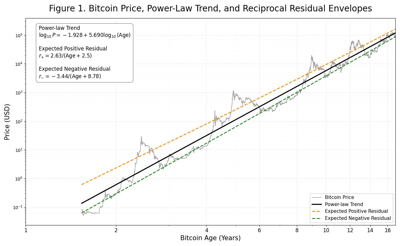
For this article we use a two-sided residual model with reciprocal decay to estimate the expected magnitude of positive and negative deviations from Bitcoin’s long-term power-law trend. These estimates are then converted into local volatility and age-adjusted Z-scores, allowing every point in Bitcoin’s history to be expressed as a comparable percentile.
But you say, why not just look up recent one-year volatility and take it from there? It’s probably fine in many instances, but an age-adjusted residual method takes into account the full Bitcoin history and long-term scaling. It evolves the volatility value smoothly as Bitcoin matures and allows deviations from different eras to be compared on the same statistical scale.
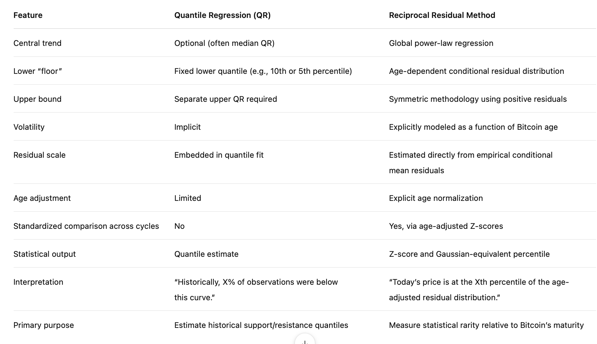
Quantile regression is one valid method of looking at percentile levels; the reciprocal of Bitcoin age residual method used here is a different approach, and the table below outlines the differences between the two approaches.
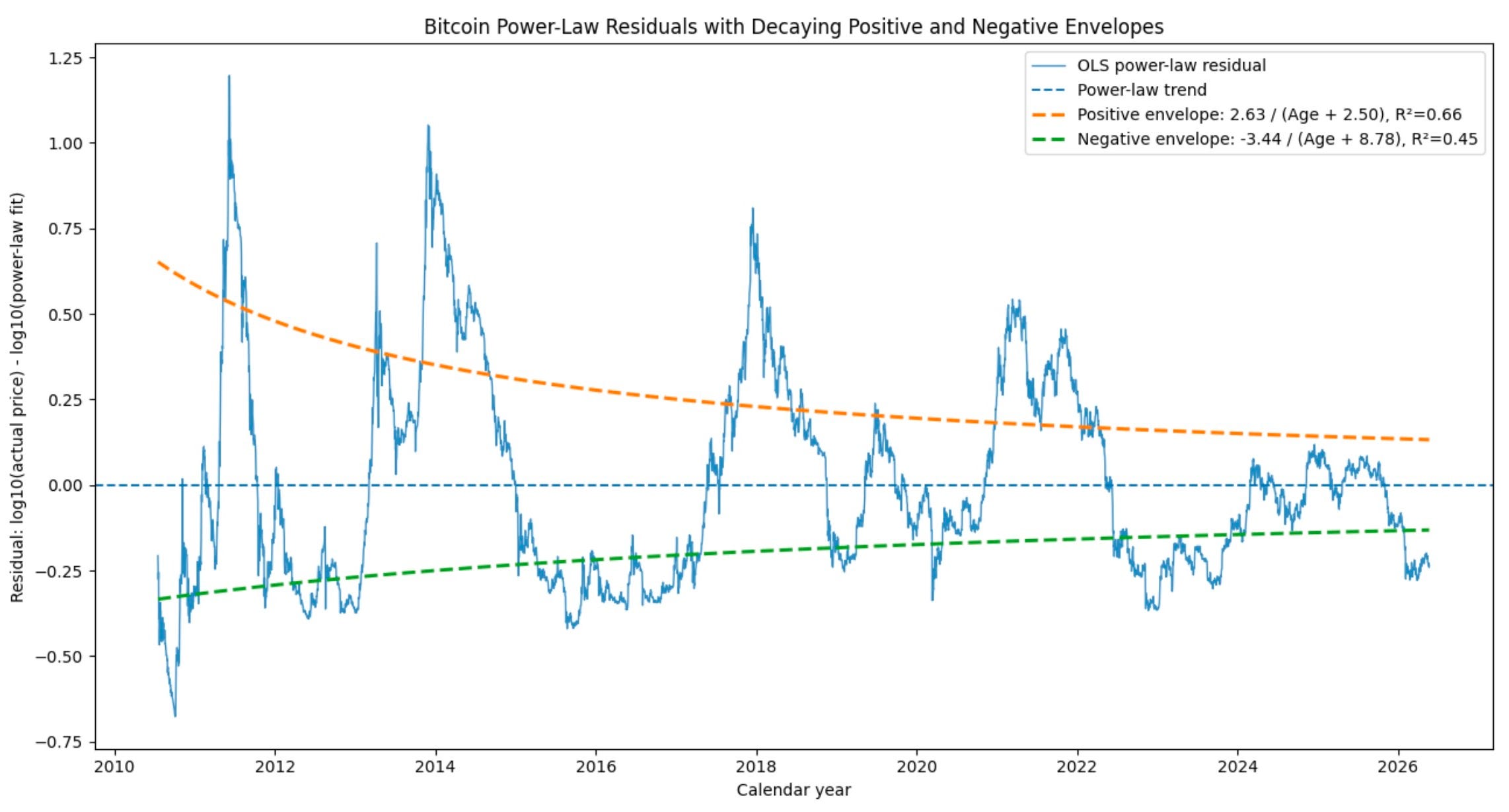
In a previous article, Bitcoin’s Two Leashes, I showed that the residuals on either side of the power law trend can be reasonably modeled by two log-normal distributions, at least for purposes of ordering and normalized Z-scores. The residuals overall skew positive and are narrower than normal (possess negative kurtosis). However dual log-normals, one for each side of the power law trend, provide a reasonable approximation, allowing us to remove most of the age dependence of the volatility, and estimate percentage levels.
7 Steps to a Percentile
We now have the background and ingredients for a 7-step procedure to calculate a Z-score for a given day and price level.
Step 1
Calculate Bitcoin age and log age. Example: If today is July 3, 2026, Bitcoin is 17.5 years old.
Log age = log10 (17.5) = 1.243. All logs are log10 herein.
Step 2
Calculate the power-law price.
log P_{PL} = -1.928 + 5.690*log (Age) = -1.928 + 5.69*1.243 = 5.145.
Price = 10^5.145 = $139,637, on power law trend at age 17.5.
Step 3
Calculate the residual for the price level. Example $58K; log P = log10(58000) = 4.763
r = log P - log P_{PL}= 4.763 - 5.145 = -0.382
Step 4
Determine which reciprocal equation to use.
If residual > 0 use:
E(r|r>0) = 2.63 / (Age+2.5)
otherwise, as in our present case:
E(r|r<0) = -3.44 / (Age+8.78) = 3.44/(17.5+8.78) = 0.131
Step 5
Convert the conditional mean residual to an equivalent σ (sigma). Assuming the positive and negative residuals are approximately half-normal, the standard deviation σ is estimated from the mean by multiplying by a factor equal to the square root of π/2 = 1.253. Thus the resulting
σ = 0.131*1.253 = 0.164 .
Step 6
Calculate:
Z = r / σ = -0.382 / 0.164= -2.329
Step 7
Convert Z to a percentile. One can use a table (or ask AI), it turns out for Z = -2.33 we are at the 1% percentile exactly. A Z-score vs. percentile level table is below.
In other words, at $58,000 and if one is at the beginning of July 2026, only about 1% of the history has been as deeply below the power-law trend, after accounting for Bitcoin’s age to normalize Z-values.
Bitcoin is at the 1st percentile of its age-adjusted residual distribution. That is a much more informative statement than saying Bitcoin has “broken the floor.” There is no single floor; there is a probability distribution.
Summary
A power law is the center of an age-dependent probability distribution. The seven-step procedure above converts any Bitcoin price into an age-adjusted Z-score and Gaussian-equivalent percentile, making valuations directly comparable across Bitcoin’s entire history.
Z-score Percentile Levels
Z-score: Normal Equivalent Percentile
+3.0 99.87%
+2.5 99.38%
+2.0 97.72%
+1.5 93.32%
+1.0 84.13%
+0.5. 69.15%
0.0. 50.00%
-0.5. 30.85%
-1.0 15.87%
-1.5 6.68%
-2.0 2.28%
-2.5. 0.62%
-3.0. 0.13%
Disclaimer: This article is for educational and informational purposes only and should not be construed as investment, financial, legal, or tax advice. The methodology described is a statistical framework for interpreting Bitcoin’s historical deviations from a long-term power-law trend and does not predict future prices or guarantee investment outcomes.
About the Author: Stephen Perrenod is Associate Director of the Scientific Bitcoin Institute (SBI), a not-for-profit organization dedicated to research and education on Bitcoin, economics, and complex systems. The views expressed here are his own.
Comments
Nothing yet. Say the first thing.
Sign in to join the conversation.