
📖 For the best reading experience with properly rendered equations, view this article on GitHub Pages.
Here’s a trick that appears everywhere in numerical computing:
Don’t solve the hard problem. Transform it into an easy one.
Multiplying a thousand small probabilities? You’ll underflow to zero. But add their logarithms, and everything works.
Convolving two signals of length n? That’s O(n²). But multiply in Fourier space, and it’s O(n log n).
These aren’t clever hacks. They’re instances of a general principle: the right domain makes computation tractable.
A domain transformation moves computation from one space to another:
Hard problem in Space A → transform → Easy problem in Space B
The pattern:
Transform input to the easier domain
Compute in that domain
Transform back (if needed)
This is worthwhile when:
cost(transform) + cost(easy computation) + cost(inverse) < cost(hard computation)
Often dramatically so.
The most common domain transformation in ML.
You’re computing the probability of a sequence:
P(x₁, x₂, …, xₙ) = ∏ᵢ P(xᵢ | x<ᵢ)
Each factor is less than 1. Multiply 1000 of them:
>>> 0.1 ** 1000
0.0  # Underflow
The true answer isn’t zero—it’s just smaller than the smallest representable float.
Work in log-space:
log P = Σᵢ log P(xᵢ | x<ᵢ)
Multiplication becomes addition. Products of tiny numbers become sums of negative numbers.
>>> import math
>>> 1000 * math.log(0.1)
-2302.58...  # No underflo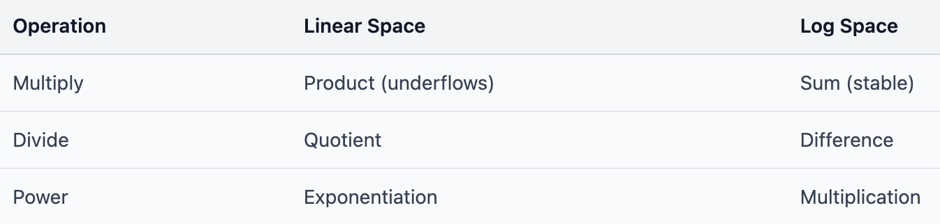
This is why every language model outputs log-probabilities. Why Bayesian inference uses log-likelihoods. Why HMMs compute in log-space.
Logarithms don’t just prevent underflow. They turn an unstable operation into a stable one.
But what if you need to add probabilities, not multiply them?
For mutually exclusive events:
P(A or B) = P(A) + P(B)
In log-space, this becomes:
log(eᵃ + eᵇ)
where a = log P(A) and b = log P(B). This comes up constantly—marginalizing over hidden states in HMMs, summing over paths in CTC, computing partition functions.
>>> import math
>>> a, b = -1000, -1001
>>> math.log(math.exp(a) + math.exp(b))
# math.exp(-1000) = 0.0 (underflow)
# Result: undefined
Exponentiating large negative numbers underflows. We’re back where we started.
Factor out the maximum:
log(eᵃ + eᵇ) = max(a, b) + log(1 + e^(−|a−b|))
The exponent −|a−b| is always ≤ 0, so e^(−|a−b|) ≤ 1. No overflow, and the underflowed term is added to 1, so we don’t lose precision.
def log_sum_exp(a, b):
    max_val = max(a, b)
    return max_val + math.log(math.exp(a - max_val) + math.exp(b - max_val))
For vectors:
logsumexp(x) = max(x) + log Σᵢ exp(xᵢ − max(x))
This is exactly what softmax uses internally:
softmax(x)ᵢ = exp(xᵢ − logsumexp(x))
The log-sum-exp trick keeps computation in log-space while handling addition.
Another profound domain transformation.
Convolution in the spatial domain:
(f ∗ g)[n] = Σₘ f[m] · g[n−m]
For signals of length N, this is O(N²)—N outputs, each summing over N terms.
The Fourier transform has a remarkable property:
ℱ(f ∗ g) = ℱ(f) · ℱ(g)
Convolution in space = multiplication in frequency.
The algorithm:
def fast_convolve(f, g):
    F_f = fft(f)        # O(n log n)
    F_g = fft(g)        # O(n log n)
    F_result = F_f * F_g  # O(n) - element-wise
    return ifft(F_result) # O(n log n)
Total: O(n log n) instead of O(n²).
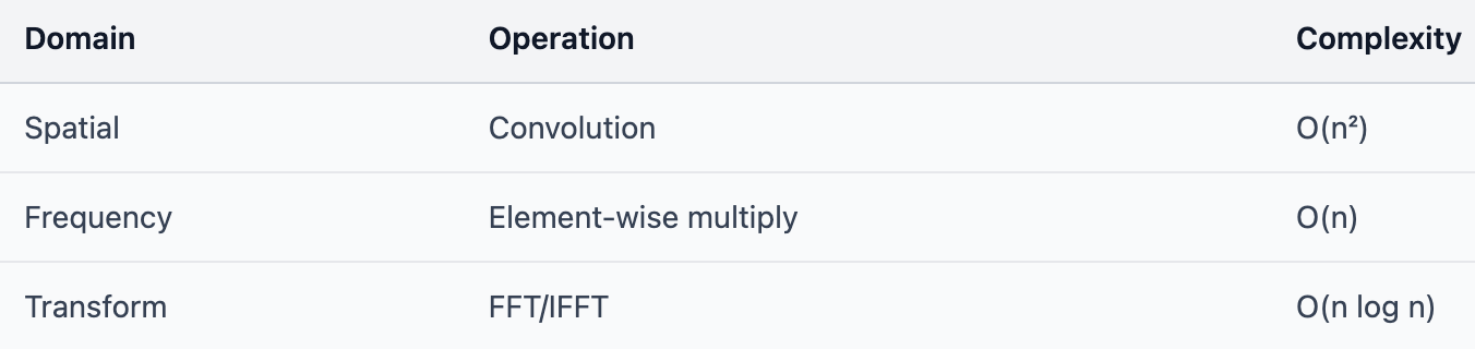
For large kernels, the transform cost is negligible. For small kernels (3×3, 5×5), direct convolution is faster—the transform overhead dominates.
In practice, modern deep learning frameworks use highly optimized direct convolution (cuDNN) even for medium-sized kernels, because GPU implementations are so fast. But FFT-based convolution remains important in signal processing and for very large kernels.
Attention looks like it should benefit from FFT:
Attention = softmax(QKᵀ)V
The QKᵀ multiplication is O(n²d) for sequence length n.
But there’s a catch: attention isn’t convolution.
Convolution is translation-equivariant—shift the input, shift the output. The kernel slides uniformly.
Attention is content-based—each position attends differently based on what’s there, not where it is.
The Fourier transform exploits the structure of convolution. Attention doesn’t have that structure.
(Some efficient attention methods like Performers and Linear Attention do use kernel approximations—but they’re approximating attention, not computing it exactly via FFT.)
A different kind of domain transformation.
Words are categorical—there’s no natural arithmetic on them.
“king” - “man” + “woman” = ???
With one-hot encoding, words are orthogonal vectors in a 50,000-dimensional space. No similarity, no structure.
Learn a dense embedding:
word → embed → ℝᵈ
Now:
embed(”king”) − embed(”man”) + embed(”woman”) ≈ embed(”queen”)
The transformation creates structure that wasn’t there before.

This isn’t just dimensionality reduction. It’s finding a space where the hard problem (word relationships) becomes easy (vector arithmetic).
Sometimes the solution isn’t a lower-dimensional space—it’s a higher one.
Data isn’t linearly separable:
Copy
         ○   ○   ○
       ○           ○
     ○    ●  ●  ●    ○
     ○    ●  ●  ●    ○
     ○    ●  ●  ●    ○
       ○           ○
         ○   ○   ○
  No linear boundary separates ● from ○.
The inner class is surrounded. No line can divide them.
Map to a higher-dimensional space where it is linearly separable:
φ: ℝᵈ → ℝᴰ where D > d
For the concentric pattern, add just one feature: z = x² + y² (squared distance from center). Now the inner class has small z, the outer class has large z. A horizontal plane separates them.
The kernel trick computes dot products in the lifted space without explicitly computing the transformation:
K(x, y) = ⟨φ(x), φ(y)⟩
For the RBF kernel:
K(x, y) = exp(−‖x − y‖² / 2σ²)
This implicitly works in an infinite-dimensional space, but you never compute it directly.
The kernel trick is a domain transformation you don’t have to pay for.
Graph Laplacians transform graph problems into linear algebra.
Clustering nodes in a graph based on connectivity. Community detection. Graph partitioning.
These seem like discrete, combinatorial problems.
Compute the graph Laplacian:
L = D − A
where D is the degree matrix and A is the adjacency matrix.
The eigenvectors of L embed nodes into Euclidean space:
nodeᵢ → (v₁(i), v₂(i), …, vₖ(i))
In this space, k-means clustering solves the graph partitioning problem.
A discrete optimization problem becomes a tractable eigenvector computation.
Many domain transformations exist for numerical reasons:
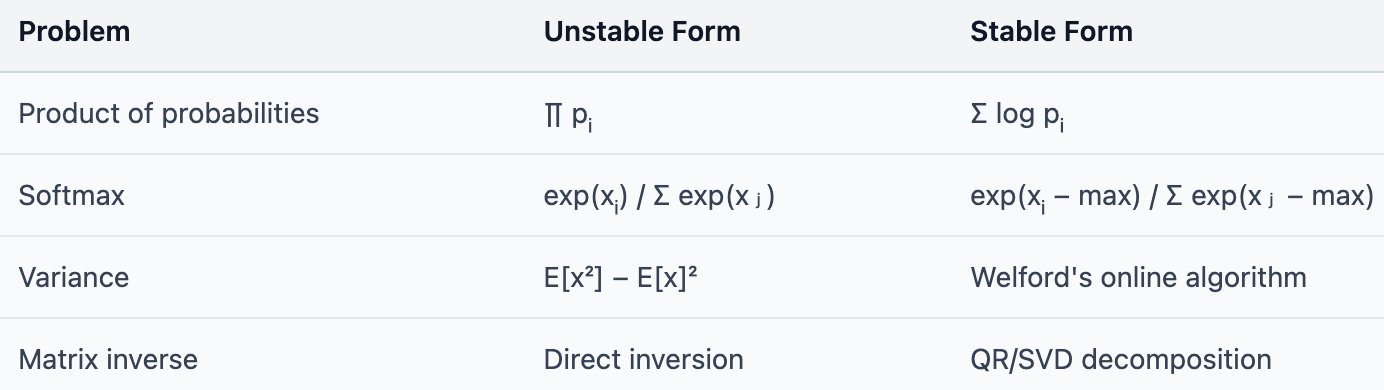
Each is a domain transformation that trades mathematical equivalence for numerical stability.
Equivalent in exact arithmetic. Different in floating-point.
The pattern recurs:
Multiplication → Addition: Use logarithms
Convolution → Element-wise: Use Fourier
Non-linear → Linear: Use kernel methods
Discrete → Continuous: Use spectral methods
High-dimensional sparse → Low-dimensional dense: Use embeddings
The skill is recognizing when your hard problem has an easier dual.
Questions to ask:
What’s expensive or unstable? Products of small numbers? Convolution? Non-linear optimization?
Is there a standard transform? Log, Fourier, Laplace, embeddings?
Does the transform preserve what you need? Some transforms lose information.
Is the round-trip worth it? Transform cost + easy computation < hard computation?
The previous articles in this series covered:
Associativity: Enables chunking, parallelization, streaming
Commutativity: Enables reordering, permutation invariance
Linearity: Enables batching, gradient accumulation
Domain transformations are different. They’re not about properties of operations—they’re about choosing the right space.
But the connection is deep: transforms often work because they reveal simpler structure.
Fourier reveals that convolution is pointwise in frequency space
Logarithms reveal that multiplication is additive in log space
Embeddings reveal that semantic relationships are approximately linear in embedding space
The transform finds a space where the problem has the structure you need.
Don’t solve the hard problem directly. Ask: is there an easier space?
Products underflow → work in log space
Convolution is O(n²) → work in frequency space
Data isn’t linearly separable → work in kernel space
The transform might cost something. But if the computation in the new space is dramatically cheaper, you win.
This is computational judo: using structure to redirect effort. The best algorithms don’t fight the problem—they find the space where the problem solves itself.
See also:
The One Property That Makes FlashAttention Possible — Associativity
Why Transformers Need Positional Encodings — Commutativity
Why Batching Works — Linearity
Numerical Recipes, Ch. 12-13 — FFT and spectral methods
Murphy, “Probabilistic Machine Learning” — Log-space computation throughout
Scholkopf & Smola, “Learning with Kernels” — Kernel methods and feature spaces
Von Luxburg, “A Tutorial on Spectral Clustering” — Graph Laplacians and embeddings
No posts
Comments
Nothing yet. Say the first thing.
Sign in to join the conversation.