Sparsity: The License to Skip

📖 For the best reading experience with properly rendered equations, view this article on GitHub Pages.

Mixtral has 46.7 billion parameters but only uses 12.9 billion per token.

It activates 2 of its 8 expert networks, leaving 72% of its weights untouched on every forward pass. This should be wasteful. Instead, it matches Llama 2 70B while running at the cost of a 13B model.

The trick is a property called sparsity.

A matrix is sparse if most of its elements are zero:

sparsity = number of zeros / total elements

A 90% sparse matrix has 9 zeros for every nonzero value.

Why should this help? Consider matrix-vector multiplication:

yᵢ = Σⱼ Wᵢⱼ xⱼ

If Wᵢⱼ = 0, that term contributes nothing. Skip it.

With 90% sparsity, you skip 90% of the multiplications. 10x speedup, right?

Not quite. There’s a catch.

Here’s the uncomfortable truth: GPUs don’t care about your zeros.

GPUs achieve speed through parallelism—thousands of cores executing the same operation on different data. They’re optimized for dense, regular memory access patterns.

Random sparsity breaks this:

• Memory access: Sparse formats store (row, column, value) tuples. Irregular access kills cache efficiency.

• Load balancing: Some rows might have 10 nonzeros, others 1000. Cores sit idle waiting for stragglers.

• Branching: Checking “is this zero?” adds overhead.

The result: you typically need >90% sparsity before unstructured sparse operations beat dense on a GPU. And even then, the gains are modest.

The math says skip. The hardware says “I don’t know how.”

The solution: constrain your sparsity pattern so hardware can exploit it.

NVIDIA’s Ampere architecture introduced hardware support for 2:4 sparsity: exactly 2 zeros in every group of 4 consecutive elements.

[a, 0, b, 0] [c, 0, 0, d] [0, e, f, 0] ...

This gives:

• 50% sparsity (2 of 4 are zero)

• 2x throughput on Tensor Cores

• Minimal accuracy loss (networks adapt during training)

The constraint is the feature: fixed positions mean predictable memory access, perfect load balancing, no branching.

Instead of individual zeros, zero out entire blocks:

W = | A   0   B |
    | 0   C   0 |
    | D   0   E |

Each block is either:

• Dense: Use optimized GEMM

• Zero: Skip entirely

Block sizes (32×32, 64×64) align with GPU tiles. The sparse indexing overhead amortizes across the block.

Neural networks are massively overparameterized. Many weights contribute almost nothing.

Magnitude pruning: Remove weights with smallest absolute values.

The surprising finding: you can often remove 90% of weights with minimal accuracy loss.

Frankle & Carlin (2019) showed something remarkable:

Dense networks contain sparse subnetworks (”winning tickets”) that—when trained in isolation from the same initialization—match the full network’s accuracy.

The interpretation: training a large network is really a search procedure. It finds the important subnetwork; the other weights were scaffolding.

The practical recipe:

1. Train to convergence

2. Prune smallest 20% of weights

3. Fine-tune

4. Repeat until desired sparsity

Each round finds weights that seemed important but aren’t. Iterative pruning reaches higher sparsity than one-shot.

Unstructured pruning creates random zeros—exactly what GPUs can’t exploit. Options:

• Accept the irregular memory access (works at very high sparsity)

• Use structured pruning (remove entire neurons, attention heads, layers)

• Prune to 2:4 patterns for hardware acceleration

ReLU creates sparsity for free:

ReLU(x) = max(0, x)

Roughly half of activations become zero in typical networks. That’s 50% sparsity in every hidden layer.

But this sparsity is dynamic—you don’t know which values are zero until you compute them. GPUs still do the full computation, then throw away negatives.

Research directions:

• Predictive gating: Predict which neurons will be zero before computing them

• Top-k activation: Only keep the k largest activations

• Dynamic sparse training: Skip provably-zero computations

These are active research areas but not yet mainstream in production.

Here’s the most elegant form of sparsity: don’t decide which weights are zero—decide which weights to use per input.

A Mixture of Experts layer:

y = Σᵢ G(x)ᵢ · Eᵢ(x)

where:

• E₁, E₂, …, Eₙ are N “expert” networks (typically MLPs)

• G(x) is a gating/routing function

• G(x) is sparse: only top-k experts get nonzero weights

With 8 experts and top-2 routing:

• Each token activates only 2 experts

• 75% of expert parameters are skipped per token

• But total model capacity is 8x larger

This is parameter sparsity at the architecture level.

Different inputs need different computations.

• “The cat sat on the mat” → language experts

• “∫ x² dx = x³/3 + C” → math experts

• deff∞():deff∞(): → code experts

Instead of one network that handles everything, you have specialists that activate on demand.

Research shows experts do specialize: different experts prefer different token types, topics, and patterns. The routing learns to match inputs to expertise.

Switch Transformer (Google, 2021): Simplified MoE with top-1 routing. Scaled to 1.6 trillion parameters.

Mixtral 8x7B (Mistral, 2023):

• 8 experts per layer

• Top-2 routing per token

• 46.7B total parameters

• 12.9B active per forward pass

• Matches Llama 2 70B at 5x less compute

GPT-4: Reportedly uses MoE architecture.

Gemini: Uses MoE.

The pattern is clear: frontier models use conditional computation.

Full attention is O(n²) for sequence length n. At 100K tokens, that’s 10 billion attention computations per layer.

Sparse attention reduces this by only attending to a subset of positions.

Each position attends only to nearby positions:

Position i attends to: [i-w, ..., i-1, i, i+1, ..., i+w]

Complexity: O(n · w) where w is window size.

This works because most relevant context is local. Long-range dependencies exist but are rarer.

Add periodic global attention:

Position i attends to:
- Local: [i-w, ..., i+w]
- Global: [0, k, 2k, 3k, ...] for some stride k

Captures both local detail and global structure.

FlashAttention changed the calculus. By making exact attention memory-efficient, it reduced pressure for approximate sparse methods.

Modern LLMs typically use:

• Short context: Full attention with FlashAttention

• Long context: Sliding window + some global tokens

• Very long context: Hierarchical or chunked approaches

Sparse attention is less about compute savings and more about memory constraints at extreme sequence lengths.

All forms of sparsity share one insight:

Not all computation is equally valuable. Skip the parts that don’t matter.

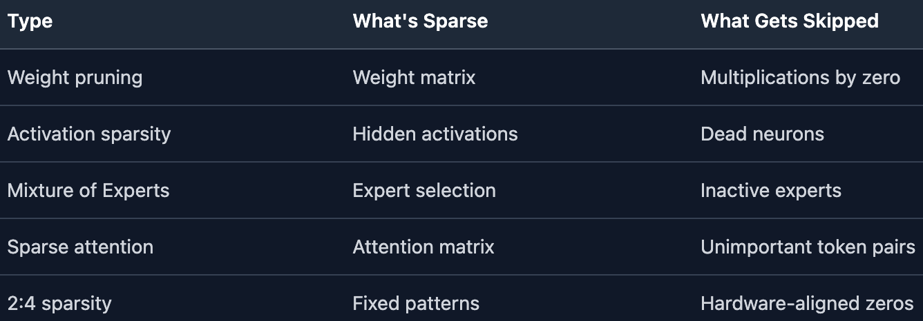
The challenge is always: turning mathematical sparsity into actual speedup.

The solution is always: structure. Align your sparsity with hardware.

Why can you remove 90% of weights without destroying the model?

Overparameterization: Neural networks have far more parameters than strictly necessary. This excess provides:

• Easier optimization (smoother loss landscape)

• Implicit regularization

• Robustness to initialization

Once trained, much of this capacity is redundant.

The Lottery Ticket View: Training is search. The dense network explores many possible subnetworks. Most are dead ends; one is the solution. Pruning removes the dead ends.

The MoE View: Different inputs need different parameters. A dense network wastes capacity using the same weights for all inputs. Experts specialize, using total capacity more efficiently.

Sparsity is the mathematical license to skip computation.

If Wᵢⱼ = 0 or unused, then skip Wᵢⱼ · xⱼ

But hardware doesn’t exploit random zeros. Unstructured sparsity gives unstructured memory access, which GPUs hate.

The practical path:

• 2:4 structured sparsity: 2x speedup with hardware support

• Block sparsity: Dense blocks, sparse selection

• Mixture of Experts: Let the input decide what to compute

The most powerful form isn’t pruning—it’s conditional computation. MoE achieves massive parameter counts with modest compute by activating only what’s needed.

This is why Mixtral matches models 5x its active compute. Having idle parameters isn’t waste—it’s the whole point. Different inputs use different parameters. No single forward pass needs them all.

Sparsity says: you don’t have to compute everything.
Structure says: here’s how to actually skip it.
MoE says: let the input decide what matters.

Previous article: Domain Transformations: The Art of Finding Easier Spaces

• Frankle & Carlin, “The Lottery Ticket Hypothesis” (2019) — Sparse subnetworks from initialization

• Fedus et al., “Switch Transformers” (2021) — Scaling MoE to trillions of parameters

• NVIDIA, “Accelerating Sparse Deep Neural Networks” (2021) — 2:4 structured sparsity on Ampere

• Jiang et al., “Mixtral of Experts” (2024) — State-of-the-art open MoE

• Pool & Yu, “Accelerating Transformer Pre-training with 2:4 Sparsity” (2024) — Training with structured sparsity