
In 1945, mathematician George Polya published How to Solve It, a slim book that became one of the most influential works on problem-solving ever written. His central insight was deceptively simple: most hard problems are solved not through brilliance, but by recognizing their connection to problems already solved.
One of his key heuristics: “Do you know a related problem? Here is a problem related to yours and solved before. Could you use it?”
In the 1990s, Japanese engineer Eiji Nakatsu faced a difficult challenge: the Shinkansen bullet train created deafening sonic booms when entering tunnels at high speed. The solution came not from aerospace engineering, but from birdwatching. Nakatsu noticed that kingfishers dive from air into water with barely a splash—a transition between mediums, just like a train entering a tunnel. By reshaping the train’s nose to mimic the kingfisher’s beak, he eliminated the sonic boom and improved efficiency.
This article applies that same heuristic to a classic distributed systems challenge: generating unique IDs at scale.
The standard answers—UUID, database sequences, Snowflake—are well-known. But there’s a deeper design space that most discussions miss. To find it, we’ll ask Polya’s question: What related problem has been solved before?
The answer, it turns out, has been shipping with your operating system for decades.
Polya’s first step is to understand the problem completely before attempting solutions. What is the unknown? What are the constraints?
We need a function that returns identifiers with this property: no two calls, anywhere in a distributed system, ever return the same value.
Every ID generation system makes trade-offs across these dimensions:
ConstraintQuestionUniquenessCan two nodes ever generate the same ID?OrderingDo IDs reflect temporal or causal order?SizeHow many bits? (Affects storage, indexing, transmission)ThroughputHow many IDs per second per node?CoordinationHow much communication between nodes?AvailabilityCan we generate IDs during network partitions?
Most systems need uniqueness. Everything else is negotiable—but every choice has consequences.
The standard solutions are well-documented:
UUIDs offer zero coordination—any node generates 128 random bits independently. But they’re large, unsortable, and their randomness destroys B-tree locality. Every insert lands on a random leaf page.
Database auto-increment gives you perfect ordering and minimal size, but requires a round-trip to a central database for every ID. It’s a throughput bottleneck and a single point of failure.
Twitter’s Snowflake hit a sweet spot: 64 bits, time-sortable, high throughput, and minimal coordination (just a one-time machine ID assignment). Its structure—41 bits of timestamp, 10 bits of machine ID, 12 bits of sequence—became the template everyone copies.
┌─────────────────────────────────────────────────────────────┐
│                    Snowflake ID (64 bits)                   │
├─────────┬───────────────────┬─────────────┬─────────────────┤
│ 1 bit   │ 41 bits           │ 10 bits     │ 12 bits         │
│ (sign)  │ (timestamp ms)    │ (machine)   │ (sequence)      │
├─────────┴───────────────────┴─────────────┴─────────────────┤
│ ~69 years │ 1024 machines │ 4096 IDs/ms/machine             │
└─────────────────────────────────────────────────────────────┘
Snowflake is excellent. But is it the only answer? Is there a deeper pattern we’re missing?
This is where most discussions stop. We won’t.
Polya’s second step is to devise a plan. His most powerful heuristic here: “Do you know a related problem?”
Let’s think about what we’re really doing. We need to:
Hand out unique resources (IDs)
To concurrent requesters (distributed services)
With minimal coordination (for performance)
Where else have we seen this exact structure?
Memory allocators have been solving a structurally identical problem since the 1980s:
Hand out unique resources (memory addresses)
To concurrent requesters (threads)
With minimal coordination (for performance)
The mapping is direct:
ID GenerationMemory AllocationUnique IDUnique memory addressDistributed serviceThreadCentral coordinatorGlobal heapNetwork round-tripLock acquisition
Could we use this? Let’s look at how memory allocators solved it.
Google’s tcmalloc uses a three-tier hierarchy:
┌─────────────────────────────────────────────────────────────┐
│                         tcmalloc                            │
│                                                             │
│  ┌─────────────┐  ┌─────────────┐  ┌─────────────┐          │
│  │Thread Cache │  │Thread Cache │  │Thread Cache │  ...     │
│  │  (no locks) │  │  (no locks) │  │  (no locks) │          │
│  └──────┬──────┘  └──────┬──────┘  └──────┬──────┘          │
│         │                │                │                 │
│         └────────────────┼────────────────┘                 │
│                          ▼                                  │
│                  ┌───────────────┐                          │
│                  │ Central Free  │                          │
│                  │    Lists      │  ← One lock per          │
│                  │ (per size)    │    size class            │
│                  └───────┬───────┘                          │
│                          │                                  │
│                          ▼                                  │
│                  ┌───────────────┐                          │
│                  │  Page Heap    │  ← Global, but           │
│                  │               │    rarely touched        │
│                  └───────────────┘                          │
│                                                             │
└─────────────────────────────────────────────────────────────┘
The key insight: push work to the edges, coordinate only when necessary.
Thread caches handle most allocations with zero synchronization. Each thread has its own pool of objects.
Central lists refill thread caches when they’re empty. This requires locks, but happens infrequently.
Page heap provides bulk memory to central lists. Even more infrequent.
The documentation states it plainly: “when following this fast path, TCMalloc acquires no locks at all.”
This is amortized coordination. You pay the cost of synchronization once per N allocations, where N is your cache size. For memory allocators, N might be hundreds of objects. For ID generators, N can be thousands.
The pattern generalizes beyond memory:
Memory AllocatorID AllocatorThread cacheLocal ID bufferArena/Central listRegional allocatorPage heap/mmapRoot coordinatorSize classID rangeObjectIndividual ID
We’ve found our related problem. Now let’s apply it.
With the memory allocator insight in hand, we can derive multiple solutions by applying the same principles.
Instead of generating IDs one at a time (Snowflake) or from a central source (database), we pre-allocate ranges:
┌─────────────────────────────────────────────────────────────┐
│                    Slab-Based ID Allocation                 │
│                                                             │
│   Central Database:                                         │
│   ┌─────────────────────────────────────────────────────┐   │
│   │ business_tag │ max_allocated │ step_size │          │   │
│   │ orders       │ 50,000        │ 10,000    │          │   │
│   │ users        │ 1,000,000     │ 50,000    │          │   │
│   └─────────────────────────────────────────────────────┘   │
│                          │                                  │
│              Request: “Give me a range”                     │
│              Response: [50000, 60000)                       │
│                          │                                  │
│         ┌────────────────┼────────────────┐                 │
│         ▼                ▼                ▼                 │
│   ┌───────────┐    ┌───────────┐    ┌───────────┐           │
│   │ Service A │    │ Service B │    │ Service C │           │
│   │[50K, 60K) │    │[60K, 70K) │    │[70K, 80K) │           │
│   │ pos: 50847│    │ pos: 62103│    │ pos: 70002│           │
│   └───────────┘    └───────────┘    └───────────┘           │
│                                                             │
│   Local allocation: just increment a counter                │
│                                                             │
└─────────────────────────────────────────────────────────────┘
Each service instance:
Requests a range from the central database (one network call)
Hands out IDs from that range locally (zero network calls, just counter++counter++)
When exhausted, requests another range
If your range size is 10,000, you’ve reduced coordination by 10,000×.
Meituan, China’s largest food delivery platform, open-sourced their ID generator called Leaf. Its “segment mode” implements exactly this pattern, with a crucial optimization: double buffering.
┌─────────────────────────────────────────────────────────────┐
│                    Leaf Service Instance                    │
│                                                             │
│   ┌─────────────────────┐    ┌─────────────────────┐        │
│   │     Segment A       │    │     Segment B       │        │
│   │   [100000, 110000)  │    │   [110000, 120000)  │        │
│   │   current: 108,934  │    │   (ready, waiting)  │        │
│   │   ███████████░░░░   │    │   ░░░░░░░░░░░░░░░░  │        │
│   │      ACTIVE         │    │      STANDBY        │        │
│   └─────────────────────┘    └─────────────────────┘        │
│                                                             │
│   When Segment A reaches 10% remaining:                     │
│     → Background thread fetches next range into Segment B   │
│                                                             │
│   When Segment A exhausted:                                 │
│     → Atomic switch to Segment B (already loaded!)          │
│     → Background thread now loads Segment A                 │
│                                                             │
└─────────────────────────────────────────────────────────────┘
This eliminates latency spikes at range boundaries. The prefetching is triggered proactively—Leaf starts loading the next segment when the current one drops below 10% capacity.
Sound familiar? It’s exactly how CPU prefetching works. Or how a streaming service buffers the next video segment while you watch the current one. Or how jemalloc returns memory to central lists before completely exhausting local caches.
The principle is universal: anticipate needs, prefetch resources, smooth out latency.
Wins:
Near-zero coordination cost (amortized to 1/N)
Sequential IDs within each slab (excellent B-tree locality)
No clock dependency (pure counters)
Simple mental model
Loses:
No global time ordering (slab A might be issued before slab B, but contain higher IDs)
Wasted IDs on crash (uncommitted portion of slab is lost)
Central coordinator dependency (though it’s touched rarely)
What if the central coordinator becomes a bottleneck? Or a single point of failure?
Here’s where we can go deeper than existing systems. Memory allocators don’t just have two tiers—tcmalloc has three (thread cache → central → page heap), and the kernel has more below that (page allocator → buddy system → physical memory).
We can apply the same hierarchy to ID allocation.
┌─────────────────────────────────────────────────────────────┐
│                  Hierarchical ID Allocation                 │
│                                                             │
│                    ┌─────────────────┐                      │
│                    │ Root Allocator  │                      │
│                    │  [0, 2^64)      │                      │
│                    │ Grants: 2^40    │                      │
│                    └────────┬────────┘                      │
│                             │                               │
│          ┌──────────────────┼──────────────────┐            │
│          ▼                  ▼                  ▼            │
│   ┌─────────────┐    ┌─────────────┐    ┌─────────────┐     │
│   │ Regional US │    │ Regional EU │    │Regional APAC│     │
│   │ [0, 2^40)   │    │[2^40, 2^41) │    │[2^41,3×2^40)│     │
│   │ Grants: 2^24│    │ Grants: 2^24│    │ Grants: 2^24│     │
│   └──────┬──────┘    └──────┬──────┘    └──────┬──────┘     │
│          │                  │                  │            │
│    ┌─────┼─────┐           ...                ...           │
│    ▼     ▼     ▼                                            │
│  ┌───┐ ┌───┐ ┌───┐                                          │
│  │L1 │ │L2 │ │L3 │   Leaf nodes (app instances)             │
│  └───┘ └───┘ └───┘   Grants: 2^12 (4096 IDs)                │
│                                                             │
└─────────────────────────────────────────────────────────────┘
This mirrors exactly how ma≪ocma≪oc works:
Your application calls ma≪oc()ma≪oc() → thread-local fast path
Thread cache exhausted → refill from arena
Arena exhausted → mmap()mmap() or sbrk()sbrk() to kernel
Kernel → physical page allocator
Each tier handles progressively larger allocations at progressively lower frequencies.
Let’s do the math. Assume:
Leaf nodes get 4,096 IDs per range (2^12)
Regional nodes get 16 million IDs per range (2^24)
Root holds the full 64-bit space
If your system generates 1 million IDs per second globally:
The root allocator is essentially write-once infrastructure. You could run it on a napkin.
This hierarchy provides graceful degradation:
Root dies:
Regionals continue with their pre-allocated ranges
At 2^40 IDs per regional, that’s years of runway
Plenty of time to restore from backup
Regional dies:
Leaf nodes continue with their local buffers
Leaves can failover to sibling regional
Or escalate directly to root (emergency path)
Leaf dies:
Only loses its local buffer (4K IDs max)
Other leaves completely unaffected
Restart gets fresh range from regional
Compare this to Snowflake, where a clock going backward can corrupt your entire ID space, or to flat slab allocation, where the central database is touched by every node.
Just as modern allocators adjust allocation sizes based on demand, hierarchical ID allocators can adapt:
class AdaptiveAllocator:
    def __init__(self, tier, parent):
        self.tier = tier
        self.parent = parent
        self.base_chunk = BASE_SIZES[tier]
        self.current_chunk = self.base_chunk
    def request_range(self, urgency=”normal”):
        # Track consumption rate
        consumption_rate = self.ids_used / self.time_elapsed
        if urgency == “emergency” or consumption_rate > THRESHOLD:
            # We’re burning through IDs fast, request more
            self.current_chunk = min(
                self.current_chunk * 2,
                self.base_chunk * 16
            )
        elif consumption_rate < THRESHOLD / 10:
            # We’re barely using IDs, request less
            self.current_chunk = max(
                self.current_chunk / 2,
                self.base_chunk / 4
            )
        return self.parent.allocate(self.current_chunk)
A sudden traffic spike? Leaves request larger chunks. Traffic dies down? Request smaller chunks to avoid waste. The system breathes with demand.
For even more sophisticated range management, consider the buddy allocator pattern:
Initial space: [0, 2^32)
Split on demand (power-of-2 blocks):
                    [0, 2^32)
                   /         \
           [0, 2^31)        [2^31, 2^32)
           /      \              ...
    [0, 2^30)  [2^30, 2^31)
       ...         ...
Benefits:
- Easy to find appropriately-sized blocks
- Simple coalescing when ranges returned
- Enables dynamic rebalancing
When a service scales down and returns unused IDs, buddy coalescing can reclaim and redistribute them. This is overkill for most systems, but demonstrates the depth of the design space.
Now for a different approach entirely.
What if you already run a consensus system—ZooKeeper, etcd, a Raft-based database? You’re already paying for consensus. Can you get IDs for free?
In Multi-Paxos or Raft, every committed entry has a unique, monotonically increasing log index. This index is:
Unique (by definition of consensus)
Totally ordered (slot N comes before slot N+1)
Durable (replicated to a quorum)
Agreed upon (that’s what consensus means)
That’s... an ID.
┌─────────────────────────────────────────────────────────────┐
│                 Consensus Log as ID Generator               │
│                                                             │
│   Log Index:  ... | 47 | 48 | 49 | 50 | 51 | ...           │
│   Content:        |cmd |cmd |cmd |cmd |cmd |               │
│                                                             │
│   Each index IS a unique, ordered identifier                │
│                                                             │
└─────────────────────────────────────────────────────────────┘
ZooKeeper’s Sequential Znodes:
zk.create(”/ids/id-”, data, CreateMode.PERSISTENT_SEQUENTIAL);
// Returns: “/ids/id-0000000047”
// The suffix is the consensus sequence number
etcd’s Revision Number:
Every write to etcd increments a global revision. With proper batching, etcd achieves 60,000-180,000 operations per second on modern hardware.
Neon’s Log Sequence Numbers:
Neon (the serverless Postgres company) uses a Paxos-like protocol for WAL sequence numbers. Their compute nodes propose entries, safekeepers agree on ordering, and the consensus slot becomes the LSN.
Naive consensus-per-ID is slow (one round-trip per ID). But you can batch:
Time window (1ms):
  Request 1: “need an ID”
  Request 2: “need an ID”
  ...
  Request 100: “need an ID”
Leader batches into single consensus round:
  Propose: “Allocate IDs [1000, 1100)”
After commit:
  Request 1 → 1000
  Request 2 → 1001
  ...
  Request 100 → 1099
Amortized: 1 consensus round per 100 IDs
You can also pipeline—propose slot N+1 before slot N commits:
t=0: Propose slot 100 (IDs 10000-10099)
t=1: Propose slot 101 (IDs 10100-10199)  ← Don’t wait!
t=2: Propose slot 102 (IDs 10200-10299)
t=3: Commit for slot 100 arrives
t=4: Commit for slot 101 arrives
...
With batching (1000 IDs per round), pipelining (depth 4), and 2ms round-trip:
Throughput = (1000 × 4) / 0.002s = 2,000,000 IDs/sec
That’s competitive with Snowflake.
You already have it: If you’re running etcd, ZooKeeper, or a Raft-based database, ID generation is nearly free.
Strict global ordering: Unlike Snowflake (where ID 43 can be created after ID 137 across nodes), consensus gives you:
ID ordering = causal orderingClock skepticism: Edge computing, IoT, multi-cloud with NTP variance—anywhere clocks are unreliable.
Transactional semantics:
BEGIN;
  INSERT INTO orders (id, ...) VALUES (next_id(), ...);
  -- If transaction aborts, ID is never committed
  -- Can be reclaimed (unlike Snowflake)
COMMIT;
Cross-region latency: 70ms round-trip between US and EU means minimum 70ms per ID (without heavy batching). Snowflake: 0ms.
Availability during partitions: Consensus requires quorum. Network partition → minority partition can’t generate IDs. Snowflake works independently.
Simplicity: Snowflake is ~50 lines. Production Raft is ~10,000+.
The most powerful designs combine these approaches.
Use consensus to allocate ranges, then bump-pointer locally:
┌─────────────────────────────────────────────────────────────┐
│              Consensus-Backed Slab Allocator                │
│                                                             │
│                    ┌─────────────────┐                      │
│                    │  Raft/Paxos     │                      │
│                    │  Cluster (3-5)  │                      │
│                    └────────┬────────┘                      │
│                             │                               │
│           Consensus on: “Service A gets [1M, 2M)”           │
│                             │                               │
│         ┌───────────────────┼───────────────────┐           │
│         ▼                   ▼                   ▼           │
│    ┌─────────┐         ┌─────────┐         ┌─────────┐      │
│    │Service A│         │Service B│         │Service C│      │
│    │[1M, 2M) │         │[2M, 3M) │         │[3M, 4M) │      │
│    └─────────┘         └─────────┘         └─────────┘      │
│                                                             │
│    Local: counter++ (zero coordination)                     │
│    Range exhausted: back to consensus cluster               │
│                                                             │
└─────────────────────────────────────────────────────────────┘
Benefits:
Range allocations are durable and consistent (consensus)
Individual IDs are fast (local counter)
Full audit trail (”who got what range when”)
Clean failure recovery (replay consensus log)
Embed slab allocation in the Snowflake structure:
┌─────────────────────────────────────────────────────────────┐
│                  Hybrid ID (64 bits)                        │
├─────────────────┬─────────────────┬─────────────────────────┤
│ 32 bits         │ 16 bits         │ 16 bits                 │
│ Slab number     │ Timestamp       │ Sequence                │
│ (from central)  │ (seconds)       │ (local)                 │
├─────────────────┴─────────────────┴─────────────────────────┤
│ - Slabs provide rough ordering and locality                 │
│ - Timestamp within slab maintains time ordering             │
│ - Sequence handles burst within same second                 │
└─────────────────────────────────────────────────────────────┘
You get slab locality for database writes AND time ordering within slabs.
Polya’s final step: “Can you use the result or method for other problems?”
We found that memory allocators solved our problem decades ago. But the pattern is even more universal. The same structure appears across computer science:
ext4 divides disk into block groups, each with its own bitmap:
┌──────────────┐ ┌──────────────┐ ┌──────────────┐
│ Block Group 0│ │ Block Group 1│ │ Block Group 2│
│ ┌──────────┐ │ │ ┌──────────┐ │ │ ┌──────────┐ │
│ │ Bitmap   │ │ │ │ Bitmap   │ │ │ │ Bitmap   │ │
│ │ Inodes   │ │ │ │ Inodes   │ │ │ │ Inodes   │ │
│ └──────────┘ │ │ └──────────┘ │ │ └──────────┘ │
└──────────────┘ └──────────────┘ └──────────────┘
Local allocation within groups, minimal global contention. Same pattern.
Kafka partitions have independent offset sequences:
Partition 0: [0, 1, 2, 3, 4, ...]  ← Sequential within
Partition 1: [0, 1, 2, 3, ...]     ← Independent sequences
Partition 2: [0, 1, 2, ...]        ← No cross-partition ordering
Same pattern: per-partition sequencing, no global coordination.
Parallel schedulers give each worker a local queue. When empty, steal from others:
Worker A: [████] Worker B: [ ] ← steal → Worker C: [████████]Same pattern: local resources, coordinate only when necessary.
CockroachDB’s HLC combines physical and logical time:
┌─────────────────────────┬───────────────────────────┐
│ Physical (wall clock)   │ Logical (counter)         │
└─────────────────────────┴───────────────────────────┘
Stays close to real time, but logical component ensures causality. Hybrid approach—same principle.
All these domains solve the same fundamental problem: distributing access to a shared resource while minimizing coordination.
The solution is always some variant of:
Hierarchy — Multiple tiers with different granularities
Locality — Push work to the edges
Batching — Amortize coordination costs
Prefetching — Anticipate needs before they arise
These patterns were discovered in OS research in the 1970s-80s. They were refined in memory allocators through the 90s-2000s. And they apply directly to distributed systems today.
There’s a deeper reason why memory allocator patterns work for distributed ID generation: parallel programming is a special case of distributed programming.
Both solve the same fundamental problem: independent execution units coordinating access to shared resources. The difference is in the constraints:
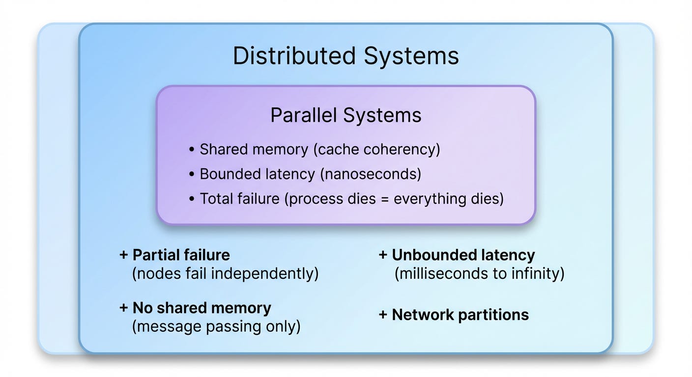
The implication: If you solve a problem under distributed constraints, the solution automatically works for parallel. But not always vice versa.
This is why tcmalloc’s patterns transfer so cleanly—the coordination avoidance principles that work across threads (where lock acquisition is expensive) also work across continents (where network round-trips are expensive). The cost function changes, but the optimization strategy remains the same.
What transfers directly:
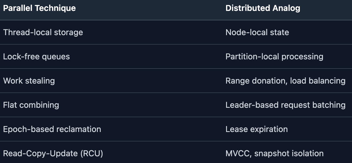
What doesn’t transfer (the “distributed tax”):
Partial failure: In parallel systems, if one thread crashes, the process dies. Clean slate. In distributed systems, Node A crashes while B and C continue—with stale views of A. This is why distributed systems need failure detectors, consensus, and replication.
Unbounded latency: The FLP impossibility result proves that deterministic consensus is impossible in asynchronous systems with even one crash failure. This fundamental limit doesn’t exist in parallel programming where timing is bounded.
No shared memory: Parallel systems get cache coherency protocols (MESI) for free. Distributed systems must build replication and consistency from scratch.
The connecting figure: Leslie Lamport. His 1978 paper “Time, Clocks, and the Ordering of Events in a Distributed System“ introduced “happens-before”—a concept that applies equally to memory models (parallel) and causality (distributed). His bakery algorithm solved mutual exclusion for threads; Paxos solved consensus for nodes. Same mind, same patterns, different constraints.
Understanding this relationship is a superpower. When you face a distributed systems problem, ask: “How did parallel programming solve this?” Often, the core insight transfers—you just need to handle partial failure and unbounded latency on top.
When should you use each approach?
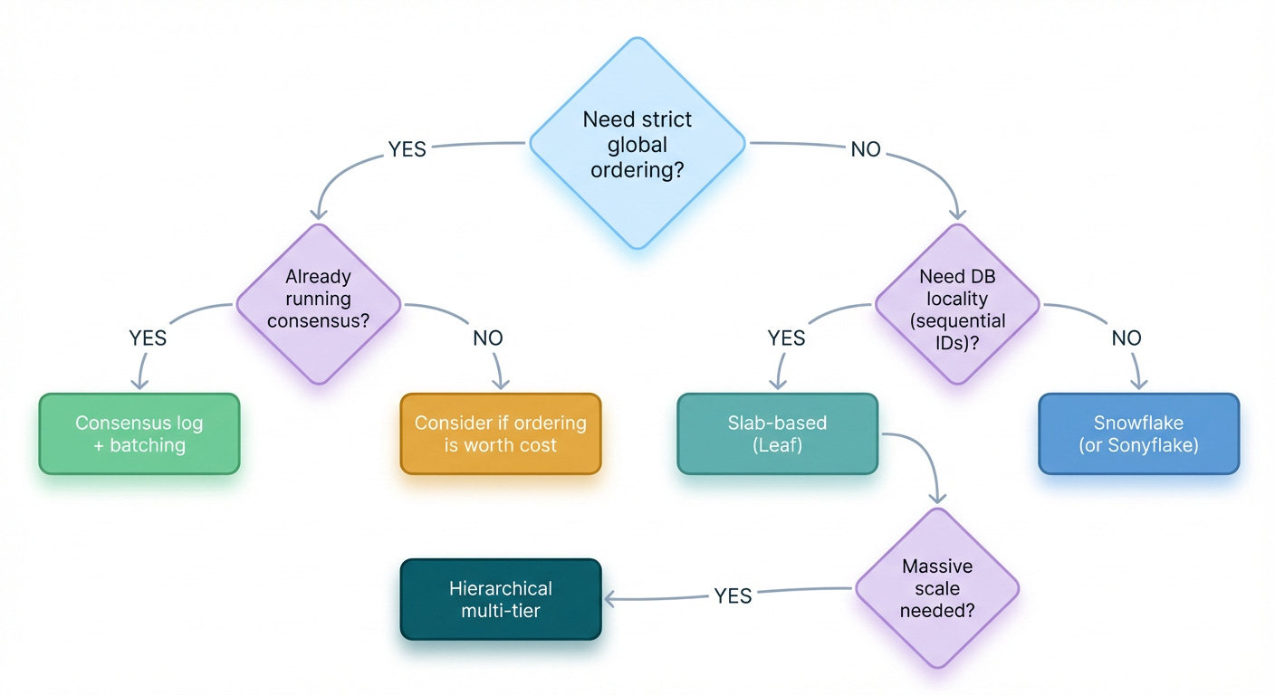
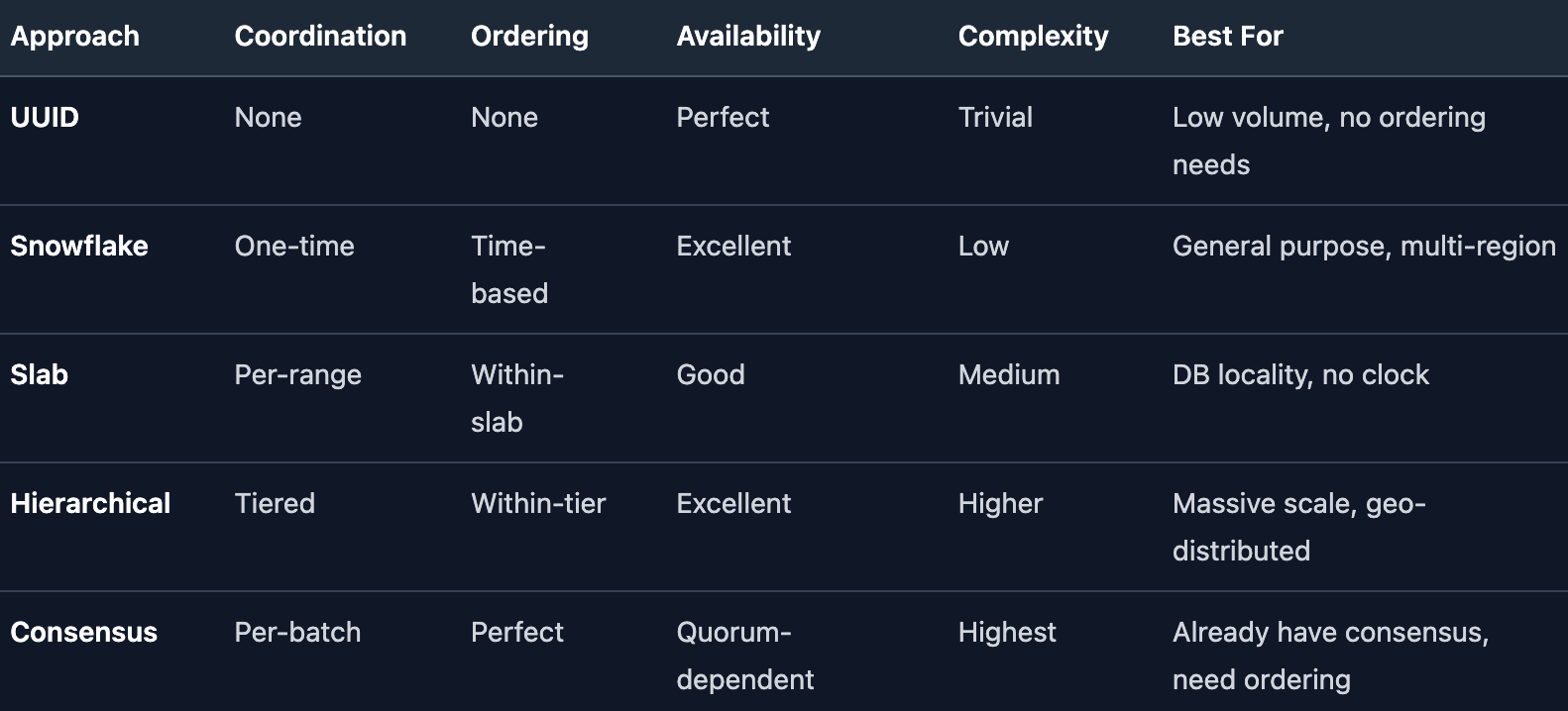
We started with a question: how do you generate unique IDs in a distributed system?
The standard answer is Snowflake. But by asking Polya’s question—“Do you know a related problem?”—we discovered an entire design space hidden behind one well-known solution.
Memory allocators solved this problem decades ago. The same patterns appear in filesystems, streaming systems, schedulers, and distributed clocks. Once you see the connection, the solutions almost derive themselves.
The deeper lesson isn’t about ID generation. It’s about problem-solving.
Next time you face a hard distributed systems problem, ask:
What is the underlying structure? (Unique resources, concurrent access, coordination cost)
What other domain solved something similar? (OS, networking, databases, hardware)
Can I extract and transfer the principle? (Hierarchy, locality, batching, prefetching)
The best engineers don’t memorize solutions. They recognize patterns.
Eiji Nakatsu saw a kingfisher dive into water and redesigned a bullet train. The principles of tcmalloc power your ID generator. The patterns are everywhere—if you know how to look.
The Pattern
TCMalloc Design — The memory allocator that inspired this thinking
Mimalloc Paper — Free list sharding and segment allocation
The Solutions
Meituan Leaf — Production slab-based ID generator
Snowflake — Twitter’s original design
Sonyflake — Variant optimized for longevity
Neon’s Paxos — Consensus for log sequence numbers
TiDB TSO — Timestamp oracle design
Spanner Sequences — Batch allocation in practice
The Parallel ↔ Distributed Connection
Time, Clocks, and the Ordering of Events — Lamport’s foundational paper explained
FLP Impossibility — Why distributed is fundamentally harder
Coordination Avoidance in Databases — Peter Bailis on when coordination is necessary
The Method
How to Solve It — Polya’s classic on problem-solving heuristics
The Shinkansen and Kingfisher — Cross-domain problem solving in action
No posts
Comments
Nothing yet. Say the first thing.
Sign in to join the conversation.