The Wave Function - Book Excerpt #17

This is section III.3 (that builds upon the previous section here) of the first volume of my book, “Quantum Physics: An Overview of a Weird World.” I plan to post regular updates, including minor and substantial revisions, on Substack. Here is the full table of contents and guidance on how to follow the book as it unfolds.

Let us return briefly to the de Broglie hypothesis. Here we had to deal with an abstract object, with a sort of conceptual synthesis that resembles quite well both a wave and the appearance of a particle. Every particle in quantum theory, like the electrons, protons, photons, etc., can be represented by a wave packet, that is, a small localized wave that travels throughout space and that has a frequency (or wavelength, if you prefer), and a maximum central value that decays quickly on both sides (recall Fig. 2). It is a way to visualize a wave that nevertheless can interact locally as a particle and conceptually synthesizes the wave-particle duality, where the quantum objects seem to behave as waves and yet as particles too.

Then, starting from Section I.2 we have also seen that in quantum mechancis we must deal with interference phenomena, which bear some similarities to that of the waves of classical mechanics. We introduced the concept of the phase between two waves, or a phase relative to an origin, and we saw how this is reflected in the formalism of quantum theory.

Now, the mathematical function which describes a wave packet or any quantum mechanical description of the state of a system is called the wave function and is usually written with the Greek letter ψ (read “Psai” for uppercase, “psi” for lowercase). The wave function contains all the information about a particle or a quantum system, for example, in space coordinates x and in time t as: ψ(x, t). This is, in fact, the conventional and standard mathematical description of waves in quantum mechanics.

In section I.3 we also found that the intensity of a wave—that is, the physical quantity that we really measure, say, the number of photons we measure arriving in a specific area on a detection screen—is given by the squared modulus of the wave function as,

where, here, we consider only the change in the space, variable x, leaving out the change in time, variable t. Therefore, it is convention to depict a wave packet as in Fig. 1.

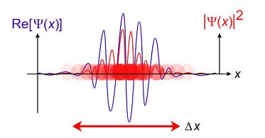
You see the real part of a wave function (the wave with positive and negative values) and its squared modulus (the wave with only positive oscillations), which represents the effectively measured intensity.1 The ∆x is taken as measuring the width of the wave packet and corresponds to the uncertainty over the position of a particle due to Heisenberg’s inequality.

If you think of the density of dots, for instance, those forming the interference fringes on the screen of the double slit experiment, the number of photons hitting per unit area the photographic plate (or a ccd camera, or whatever kind of detector), the intensity is just proportional to the density of dots. The registered number of particles on the screen per unit area (or, as it is represented graphically in this picture, like the transparency of the particle around an origin) can be taken to be proportional to the probability of finding the particle in that specific area.

Recall that while the overall disposition of many photons on the screen resembles that of the interference fringes, the site where the single particle will hit the screen is nevertheless a completely probabilistic process. The appearance of one photon as a dot on the screen is purely a statistical phenomenon.

Therefore, one can regard the intensity—that is, the squared modulus of the wave function—as something proportional to a probability per unit area, that is, a probability density. The squared modulus of the wave function is the master tool with which physicists describe probabilities in quantum mechanics, that which connects theory with experiments and observations. It is what allows an abstract complex mathematical function to correlate with reality: all the measurement processes that physicists perform in the laboratory.

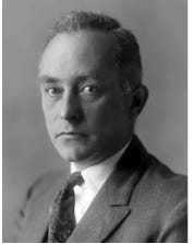
We can introduce the following interpretation, which is due to the German physicist Max Born, and which is also called the Born rule :2

The squared modulus of the wave function according to Eq. 1 is a probability density p(x) to observe a quantum system in a specific state x.

To clarify what this rule means, let us consider the graph of Fig. 3. Let us suppose that the curve represents the probability density to find a particle around an origin.

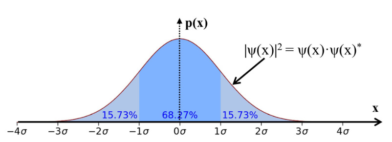
If the horizontal axis represents the position x where a particle can be found, the vertical axis is the probability density p(x) to find it at x. You will frequently find such kinds of bell-shaped curves in several textbooks; it is the normal distribution or Gaussian distribution.

However, a probability density is still not a quantity that can be measured because it represents only an infinitesimal quantity. It makes no sense to ask what the probability is of finding a particle in a specific position, as the interval on the space axis, in such a case, would be zero. One can only say with what probability a particle can be localized in a specific spatial interval around the origin (say, the x we worked with in Heisenberg’s uncertainty principle). The name “density” is no coincidence. Just think of the density of matter. The material density function of a body describes how the density varies inside its volume. Yet this still isn’t enough to tell us something about the amount of matter if we don’t specify how large the volume is and how its density function varies inside that volume. Similarly, the wave function and its associated squared modulus, the probability density, describes all the possible states of a system but still does not tell us the probability of finding it in a range of possible states. What we must consider is the sum of the probability density function over a specific range, which tells us something about the effective probability P to find it in that range.

For example, for normal distributions, the spatial x-interval of ±σ (“sigma”) is per definition the range that determines a 68.27% probability of finding a particle. σ is called the standard deviation and tells us something about the dispersion of a set of data values. The probability of finding the particle far from the center drops off quickly. At ±3σ, it is almost zero.

In general, to obtain a probability P of finding the particle inside some spatial range between x = a and x = b, we must take the integral of the probability density over that interval—that is, the integral over the squared modulus of Ψ(x). An integral is the area under the graph’s function which can be obtained as the sum over all the function’s values at each point along the x-axis, in our case:3

And, if you consider the probability of finding a particle anywhere, throughout the Universe, the spatial range must be infinite, taking a = −∞, b = +∞ as the domain of integration. Then, obviously, you will get 100% probability that is, the certainty of finding it somewhere, which mathematically translates into the integral giving unity:

The expression in the brackets on the left-hand side of the equation is simply a more compact form to express the integral. It is quite common shorthand, the so-called Dirac notation, that we will take up in more detail soon.

More generally, the wave function applies not only to a particle’s position but to any possible state. It is a calculation tool with which to also find the probability of finding a particle having a momentum or angular momentum (the rotational speed), an atom or a nucleus being in some energetic state, etc.

The takeaway message of all this is that quantum mechanics is a purely probabilistic theory. This is due to its wavy nature. There is no way of knowing how a single particle will behave, not even in principle (except when the particle is in what is called an eigenstate, as we will see later). That is why, in quantum theory, statistical tools play such an important role. We can compute the probability only to measure a value in some interval. In quantum mechanics, it makes no sense to speak of a system that is in some state. It makes sense only to say that there is a certain probability that a measurement will furnish an outcome that we associate with some state at the instant of measurement. However, we are not allowed to say anything about its state before and after that measurement. The wave function is a state function only in the sense that it is a mathematical tool that tells us about the statistics and probability of finding a specific system in a specific state or range of possible states.

The next section will tackle with the question is whether the wave function is simply an abstract mathematical description of the statistical behavior of a system that simply updates our knowledge, or whether it represents a real object in the physical world.