On Catastrophic Forgetting

For most of my career I’ve been a theoretical physicist working on normal theoretical physics problems. (Particles, strings, gravity, etc. etc.) I’ve recently been working instead in machine learning, and am slowly working my way through basic phenomena in this field.

I recently decided to write short articles on my efforts. Unlike most of my writing, I am not really sure who these words are targeted at. I suspect seasoned deep learning practitioners might find everything that I say obvious. So perhaps this is targeted more at ML-curious scientists from other disciplines. Your enjoyment may vary.

Today I’m writing about catastrophic forgetting.

In “textbook” machine learning, when building a neural network to perform a task, you first train it on some appropriate data, and then test its performance on some test set which is from more or less the same distribution. As an example, we might build a classifier by using as a training set images of handwritten digits from the well-known MNIST data set:

We train the network to take in an image and output the corresponding integer from 0 to 9. Importantly, we mix all of the digits together when presenting the training data to the network. This is a very easy problem and its trivial to solve it completely.

Now let’s try a variant on this: let’s first present images of only the digits [0,1] and train it to classify those. Then, let’s train it on the digits [2,3] alone. Will it remember how to distinguish 0s from 1s?

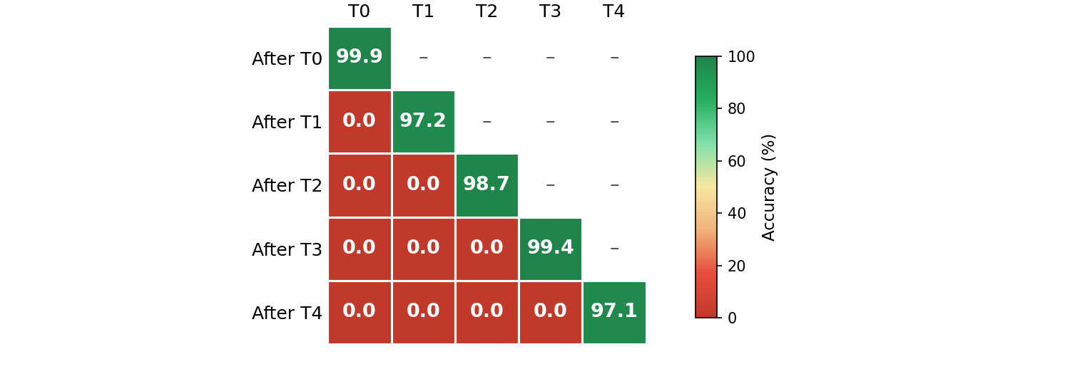
The answer is no. If you don’t take any special care, each new task that it learns makes it completely forget the old tasks. Above is my attempt at reproducing this with a simple fully connected neural network. Here “T0” is classifying [0,1], “T1” is classifying [2,3], etc. up to T4 on [8,9]. The accuracy on an old task is essentially entirely 0% after learning a new one. Note that this is worse than random chance: after learning about [2,3], the network will always assign images of [0,1] one of the most recently seen digits 2 or 3, which is exactly wrong.

This isn’t surprising. When training on T1, the network is optimizing for a different problem than T0. There is no reason for the tyranny of gradient descent to preserve any knowledge of the original task.

It’s interesting to compare this to the wildly different way that humans learn, where learning how to juggle does not immediately mean that you forget how to tie your shoelaces. There are a few obvious differences between my brain and the three layer MLP that I trained above:

1. I can do other things than classify numbers. I have a rich knowledge of the world, and in a sense each new task that I learn how to do is simply a small perturbation that uses that existing knowledge in a slightly different manner.

2. I have a memory. I confess that I don’t really know how it works, but its contents seem to be long-term and don’t appear to be dramatically altered as I learn new things.

Let’s try to solve this problem in a way that is both maximally entertaining and is inspired by the two points above.

Let’s start with point 2. It seems reasonable to try and give our network a memory. We will use a Hopfield memory, largely because as a physicist I find the energy-based construction extremely soothing.

Consider the problem of trying to store a collection of memories, where we imagine that each memory is a d-dimensional vector x, and we would like to store N of them. A Hopfield memory is a way of creating an energy function E from this set of N vectors, such that the energy is minimized at each memory vector xᵢ. To recall a memory, you first initialize your system at some other random place (call it ξ) and iteratively minimize the energy, updating ξ and searching for a minimum. If you use the memory responsibly, then you are guaranteed to end up at one of the stored patterns.

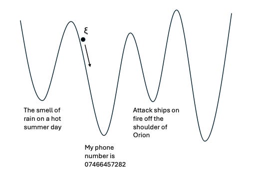
Which memory do you recall? It depends on your starting point; presumably you will end up at the memory which is geometrically closest to the starting point, under some definition of “close”. Thus if you remember half of the components of your starting memory vector and start there, initializing the missing half to zero, you will probably end up falling into an energy basin whose minimum fills in the remaining half.

In our work we will use the “modern Hopfield network”, where the precise equation for the energy is:

where X is a (N x d) matrix containing all the stored patterns.

How do we use this for our specific problem? One very brutal way is to simply force the memory to be a classifier itself. Consider flattening the 28 x 28 input images into a 784 component vector and then concatenating a one-hot vector storing the label to end up with a (784+10) dimensional “pattern”. We then store all these patterns into our Hopfield memory. To classify a new image, we treat it as a problem in pattern recall: we initialize the “image” part of the vector with the input image and ask the memory to fill in the remaining “label” part of the vector through the Hopfield dynamics.

This kind of works! You can sequentially load in the input images, and it does not catastrophically forget at all, since its core is after all a memory module and not something with weights that update. But it is also a very lousy classifier (the best I get is ~60%) for precisely the same reason. There’s no “deep learning” going on here. It is simply finding whichever label is the closest one using some notion of similarity in the 784 components of raw pixel space.

It seems that if we are going to do better we need to find a better representation of the input image.

Luckily, the building of more informative representations is a well-studied problem. We are going to do this by using a variational autoencoder (or VAE). Formally, this is a kind of generative model which you can imagine as giving you a highly compressed representation of the initial data. It takes in input x, and compresses it into a (usually) much smaller dimensional representation z which captures all the key information, in particular allowing the original input to be reconstructed. If you want more details, I refer you to this review.

The idea for us is that because it is compressed z is usually much more “enlightened”, focusing only on the relevant structure of the initial image. This is unsupervised: importantly, the VAE itself has nothing to do with classification, and doesn’t even take in the labels as input.

What data do we use to train the VAE? Even though the labels aren’t involved, I feel that according to the rules of the game we shouldn’t expose any of the MNIST data before our sequential presentation of the MNIST tasks. Instead, we will first train the VAE to reconstruct handwritten letters from the closely related ExtendedMNIST (EMNIST) dataset, which has all the letters but no numbers:

If you are a little bit poetic, this is kind of addressing Point 1 in my list of differences between a human brain and the MLP above. By training the system on a series of letters that aren’t really related to the final problem, I am giving it background knowledge on how to interpret pixels in terms of handwritten lines rather than grids of 0s and 1s. It is kind of soothingly reminiscent of human learning that the best way to train it to do this is to ask it to learn how to write its own letters by copying existing ones.

After we first train the VAE, we then “learn” to do the original digit classification task by passing each digit image through it in sequential fashion, getting a compressed z, and then store the patterns in our Hopfield memory using this compressed z (concatenated with the labels) rather than the original raw pixel data. This truly works very well. For a 20-dimensional latent state z we get the following qualitatively different performance.

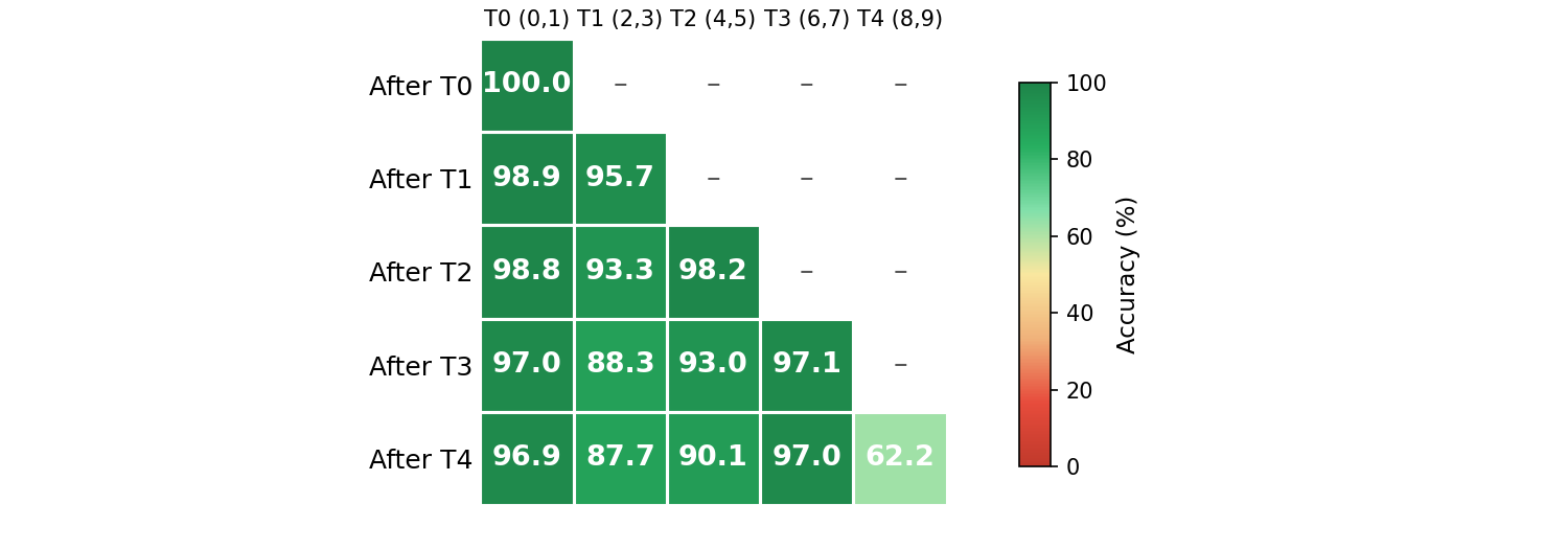
This is great!

Unfortunately, I feel that we are cheating. If you are following along closely, then you will have noticed that the modern Hopfield memory1 explicitly takes in all of the training data, meaning that in the current case we are storing a highly compressed representation of the training data in computer memory in an (N x 30) dimensional large matrix X, where N is the number of training samples. It seems somewhat disingenuous to claim success at overcoming forgetting when I’m just explicitly compressing all of the training data into memory. (On the other hand, is it? To be honest, I’m not sure. An overparametrized neural network would also do something like this internally, but it would appear much more opaque — and probably more palatable — because it would happen through the magic of gradient descent.)

In a practical application, we would have some restriction on how much memory we want to use for the problem, and ideally there should be a way to tune our approach to suit this restriction, rather than blindly storing everything.

There is a very simple way to do this. When storing each new memory x(new) into the Hopfield memory, first use it as the initial conditions for a Hopfield recall, getting an object x(closest) out. If x(closest) is close enough to x(new) (as determined by some threshold we could adjust) then we already have something in memory that is pretty close, and we probably don’t learn much from this new data point. So we don’t need to keep it.

By adjusting this threshold we can now adjust our performance on the problem depending on how much memory we have. For example, here is what we get if we adjust the threshold so we store about 12% of the initial data:

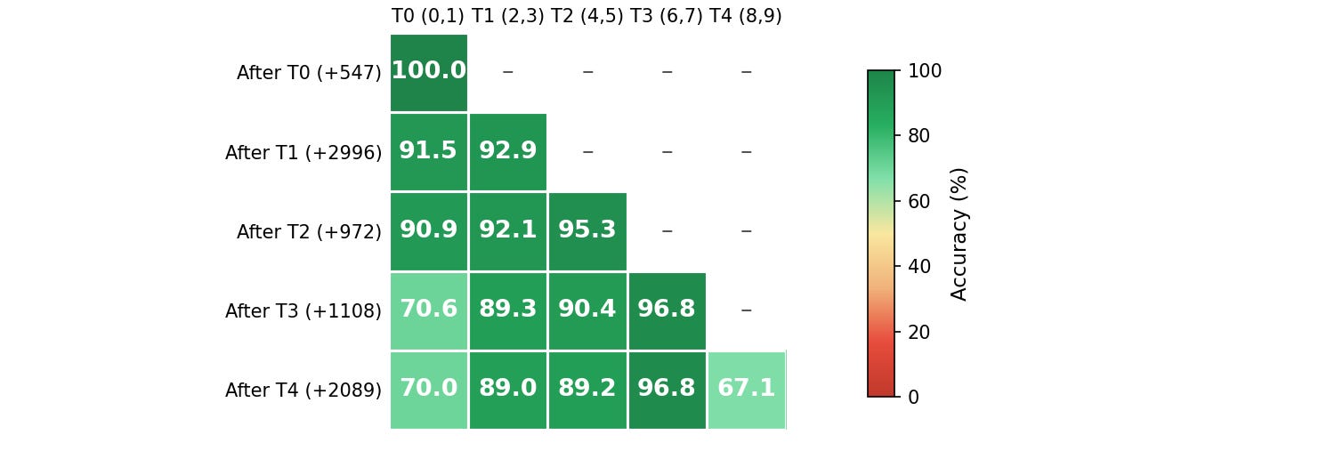
It’s worse — and it is now starting to forget things — but at least now its under our control — if we decide we want to use more memory, we do better.

There is one final missing philosophical ingredient. Note that the actual “deep learning” here is really happening at the level of the VAE. The representation of letters that it creates does not get adjusted at all as we learn the new task of recognizing each digit. In a sense the strong performance is almost an accident. This feels wrong — surely the information of the new task should backreact somehow on the stored representations.

A simple way to do this is the following: as the new stream of digit data comes in, do a few gradient steps on minimizing the reconstruction loss of the VAE using the new information. This process is now fraught with danger — if we do too many steps, then presumably everything will collapse again. But if we do it just a bit then maybe it can help a lot: the network will hopefully manage to learn things like “ah, a 9 is a lot like the familiar letter “o” except that it has a tail”, and will stop before it begins to think “omg, all that exists in the universe is the numbers 8 and 9”.

Sweeping over the number of SGD steps, the best performance I find indeed comes at an intermediate (very small) number of steps.

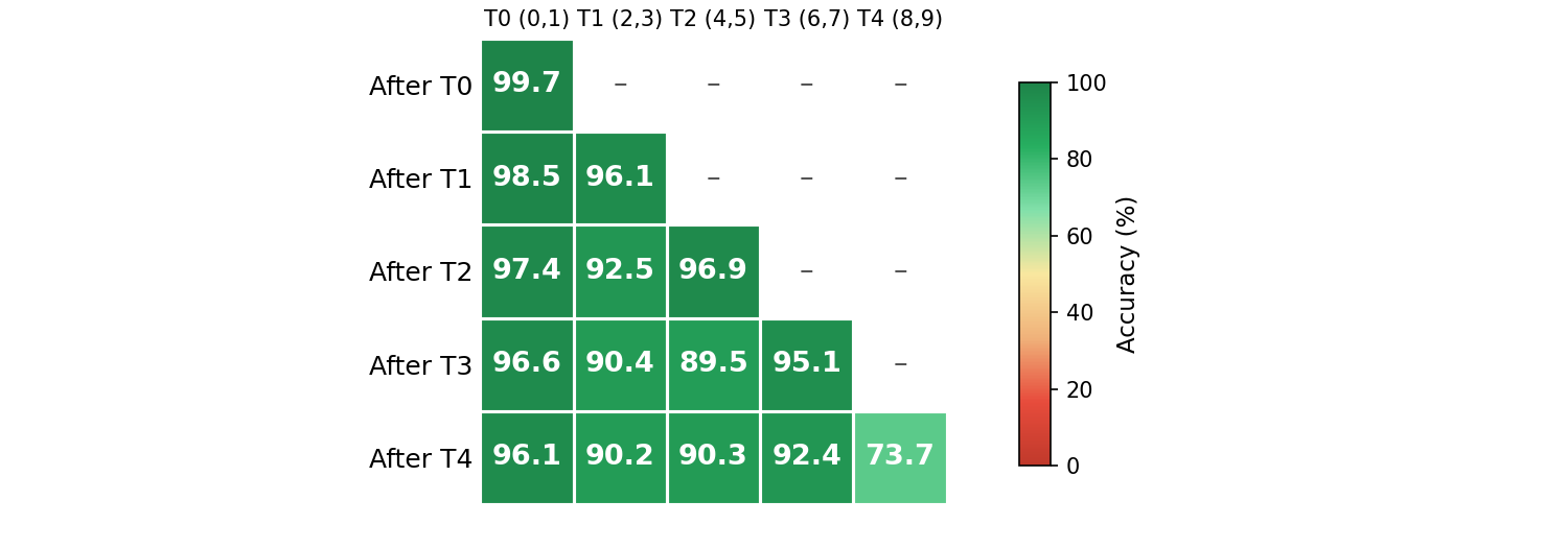
This is pretty great! Note that the collapse of task T0 from before has been completely solved.

In my eyes, this is a solution to the problem. I think this is really as much fun as one can possibly have from such a simple task, so I’m not going to push on it any more. I should stress that there are other ways to solve this, and I just focused on this path as an excuse to play with Hopfield memories and VAEs.

What are the takeaway lessons?

In a sense, we simply bolted on an extremely lightweight (and thus very controllable) Hopfield-ish classifier onto a sophisticated pretrained VAE. The problem was controllable precisely because the VAE did all of the heavy lifting and management of abstractions, and it turned out that training on the morphology of letters was enough for it to both read numbers and learn to do something different with them. There is temptation to interpret the Hopfield memory and the VAE in terms of the hippocampus and the cortex of the human brain, but because I know so little about real neuroscience I will try to resist pushing on this analogy any further.

There is something philosophically unsatisfying about the final (and in some sense most important) step, where I could not manage to make the stored representation adjust itself in a robust way. In this specific case a small and fine-tuned adjustment was enough to solve the problem we were interested in, but for genuinely difficult problems we need a way for it to safely absorb information and construct new abstractions without collapsing. Presumably there is some information-theoretical way to frame the right objective, but I don’t know what it is. (If you do, please let me know!)

I am not sure how far I will push on this, but I might next try to do something closer to actual research. A fantasy that I currently have is to try to make something more like a lightweight and crude version of a next-token prediction or language model continuously update itself, a problem which I think is genuinely very difficult. Happily, in the era of things like NanoGPT trying toy versions of such experiments seems not impossible.

All of the text of this post was written by Nabil in an old-fashioned, artisanal manner, using a keyboard. All of the experiments were run by Claude Code.