On Getting Lost In the Context and Positional Bias

I’m usually a physicist, but these days I am working in deep learning and reproducing various phenomena in simple toy models. A previous post in this series is on catastrophic forgetting.

Modern language models can store an incredible amount of information in their context, i.e. in the stream of text that they can access while generating responses. The version of Claude that I currently have open in the next tab says that its context is 200K tokens, which is about 2 average-length novels. This is an impressive amount to keep in memory, and they are growing steadily.

However, you might notice that in a long conversation, language models can sometimes get a bit confused about details. It seems that even if in principle everything fits into the context, the model can sometimes struggle to effectively recall it. Things like this are sometimes called context rot — the context “goes bad” if it goes on for long enough — and have been extensively studied.

Here’s a clean example from Figure 2 of Barbero et. al, who prompt Gemini to copy either the first or the last element in a long sequence of text. Note the interesting fact that while it can pretty much always recall the first element, it fails to recall the last one once the sequence is longer than about 300 elements. This is perhaps somewhat counter-intuitive, as it is not at all the way humans think: if someone were to suddenly reel off a phone number at me, I would probably be able to recall the last digit afterwards, but maybe not the first.

Why does this happen? In this post I’ll review one source — which arises due to basic structural features of autoregressive transformers, leading them to prefer some tokens to others -- and how to fix it in a very simple model.

The LLM is a bit opaque, and one of my goals in this series of posts is to try to illustrate everything with very simple examples that can be trained easily on a laptop. To that end, let’s think of the simplest possible model that might show an analogue of this behavior.

We will train an autoregressive transformer — where I review what those words mean below — to do the following task. Consider a sequence of tokens where each token can take one of 3 values: 0, 1, or [FLAG]. There will always only be a single [FLAG] in the sequence. The task is simply to search through the sequence for the [FLAG] and find the token immediately before it. So e.g. if we had:

0, 1, 0, 0, 0, 1, 0, 0, [FLAG], 0, 1, 1, 1, 0, 1

then the model should complete the sequence by outputting 0.

This is an extremely simple task and its very easy to make a transformer that solves it completely. To keep things interesting, I’ll make the transformer1 quite shallow (4 layers) and stop the training after only 1500 training steps, when it isn’t quite done, but is getting there.

Let’s now examine the failure rates as a function of the location of [FLAG] in the sequence. Interestingly, it looks like this:

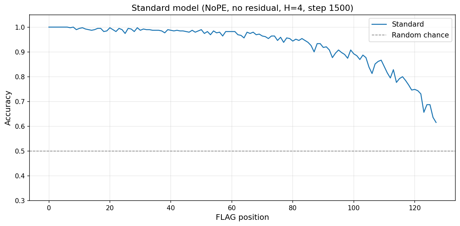
In other words, the model works correctly when [FLAG] is early on in the sequence, but gets worse and worse as it moves towards the end. This is basically the same behaviour we saw in the LLM above.

Why is this happening?

Similar things have been studied in various papers, including Barbero et. al paper, Liu et. al and others. I will focus on only one aspect of it and will follow Barbero et. al and particularly this nice recent discussion by Chowdhury, which emphasize the role of the causal masking and architectural biases.

Let’s first remind ourselves how an autoregressive transformer works. It takes in a stream of tokens, which you can imagine as a set of N vectors x, each of which is d-dimensional. The main point of a transformer is the attention mechanism, which uses some learned d x d dimensional matrices W^Q, W^K to determine how much our model’s prediction of token i should depend on token j, as captured in the N x N attention matrix A:

(where I’m suppressing factors and things of that sort). The attention matrix coordinates all interactions between tokens. Note the important fact that it is causal, i.e. that nothing appearing after token i in the sequence can affect it. This is the usual construction for language models, where the idea of the neural network is to create a conditional probability distribution that we use to sample the next letter from our knowledge of the previous ones.

Now if we think about it, this causal masking means something dramatic: tokens at the beginning of a sequence end up having a huge effect on what happens later on (because they can be seen by all subsequent tokens), but tokens towards the middle or end of the sequence have a smaller effect as they are seen by relatively fewer tokens.

Let’s understand this quantitatively by making a plot of the derivative of the final token output of a randomly initialized transformer with respect to the input token at position j as we vary the number of layers H, i.e.

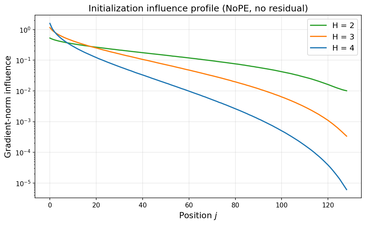
Note that this is a log scale, and the effect is very strong indeed! It becomes stronger as we increase the number of layers. For this no-residual network apparently after 4 layers the first token has ~10^6 times more influence on the final output than the last one.2

This is now starting to smell like the failure patterns we saw above: possibly the reason the network loses things from the end of the sequence is that they simply architecturally have far less influence.

One might hope that as the network trains it learns to solve this issue; indeed even in the toy example if I train it for long enough the error curve I showed above flattens out. Conceptually however it would be nice if we could fix it from the start, i.e. find a way to liberate the network from its intrinsic positional bias. I describe a way to do this below. This part of this post appears to be novel, to the best of my knowledge. However it’s really very simple and I find it quite possible it’s already out there in the literature somewhere. If a reader knows about a similar mechanism please let me know and I’ll add a citation.3

One way to fix it is to imagine deliberately offsetting it, i.e modifying the attention mechanism above like this:

where B(ij) is a matrix that we construct precisely to counteract this intrinsic bias by explicitly giving more weight to later tokens. It is a pure table of data-independent numbers, and can be computed once and for all explicitly for a given architecture. I sat down to work it out by hand and rapidly got confused; it has a combinatorical flavor with nice formulas discussed by Chowdhury , but in my actual model the presence of nontrivial things happening between the attention mechanism applications (LayerNorm, the MLPs) made it hard for me to calculate the actual numbers.

At some point I realized that actually I don’t need to calculate it by hand: I could just determine it numerically by demanding that it be chosen to flatten the influence profile above at initialization. The resulting numerical iteration converged rapidly and the output B(ij) looks like this:

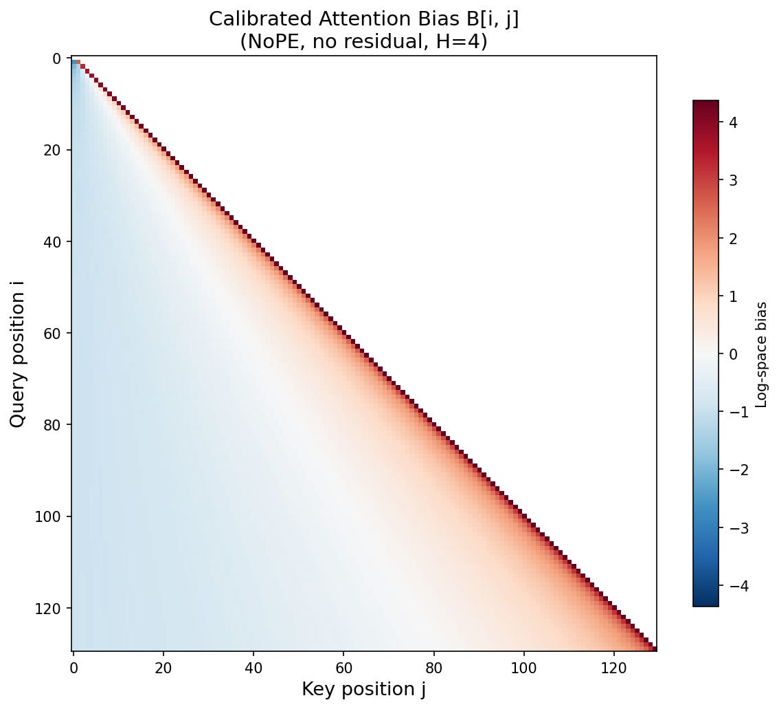
As expected, it weights later tokens much more.

Now, does it help? We can insert it into the same minimal transformer that we studied previously with the toy recall task. Happily, the resulting bias-corrected transformer trains much faster:

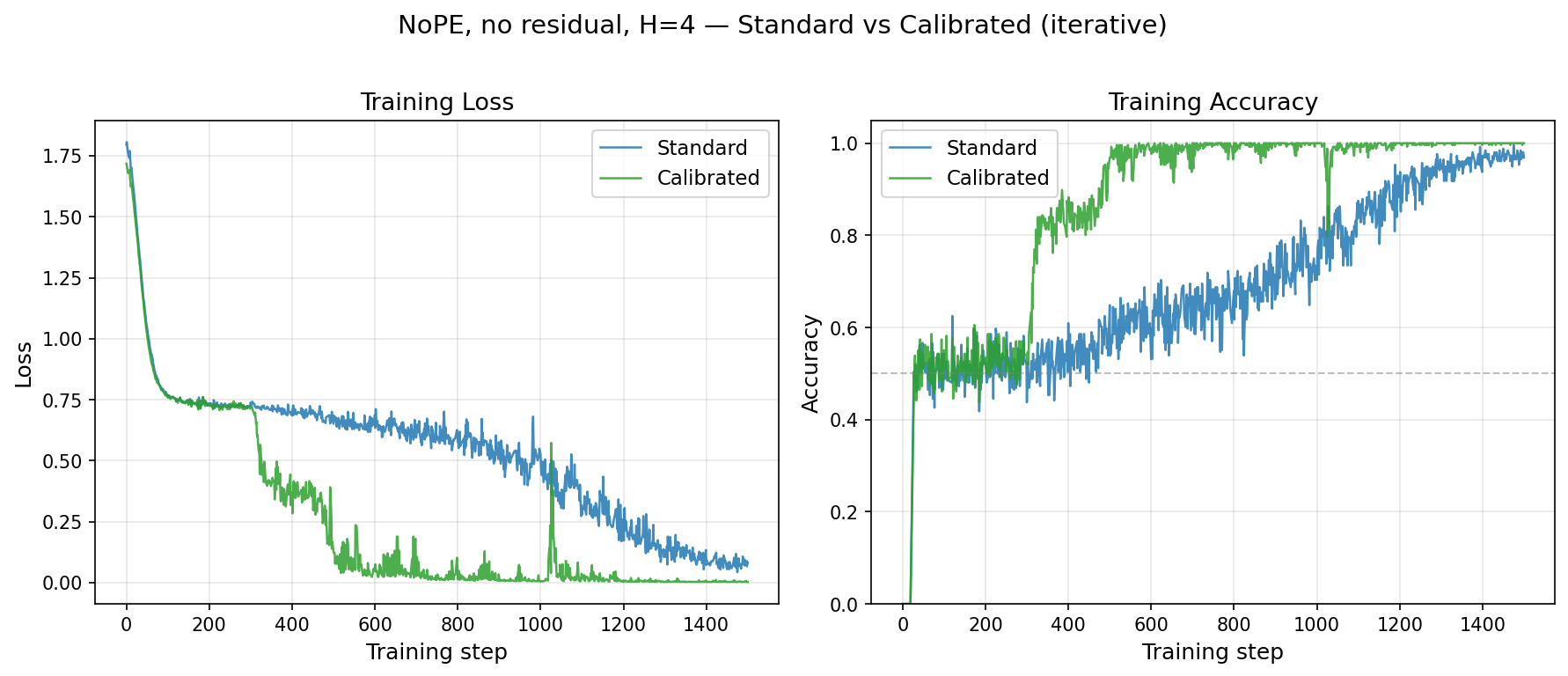
and does not have the previous preference for earlier tokens, achieving perfect recall all the way along the sequence even when the naive one was still confused:

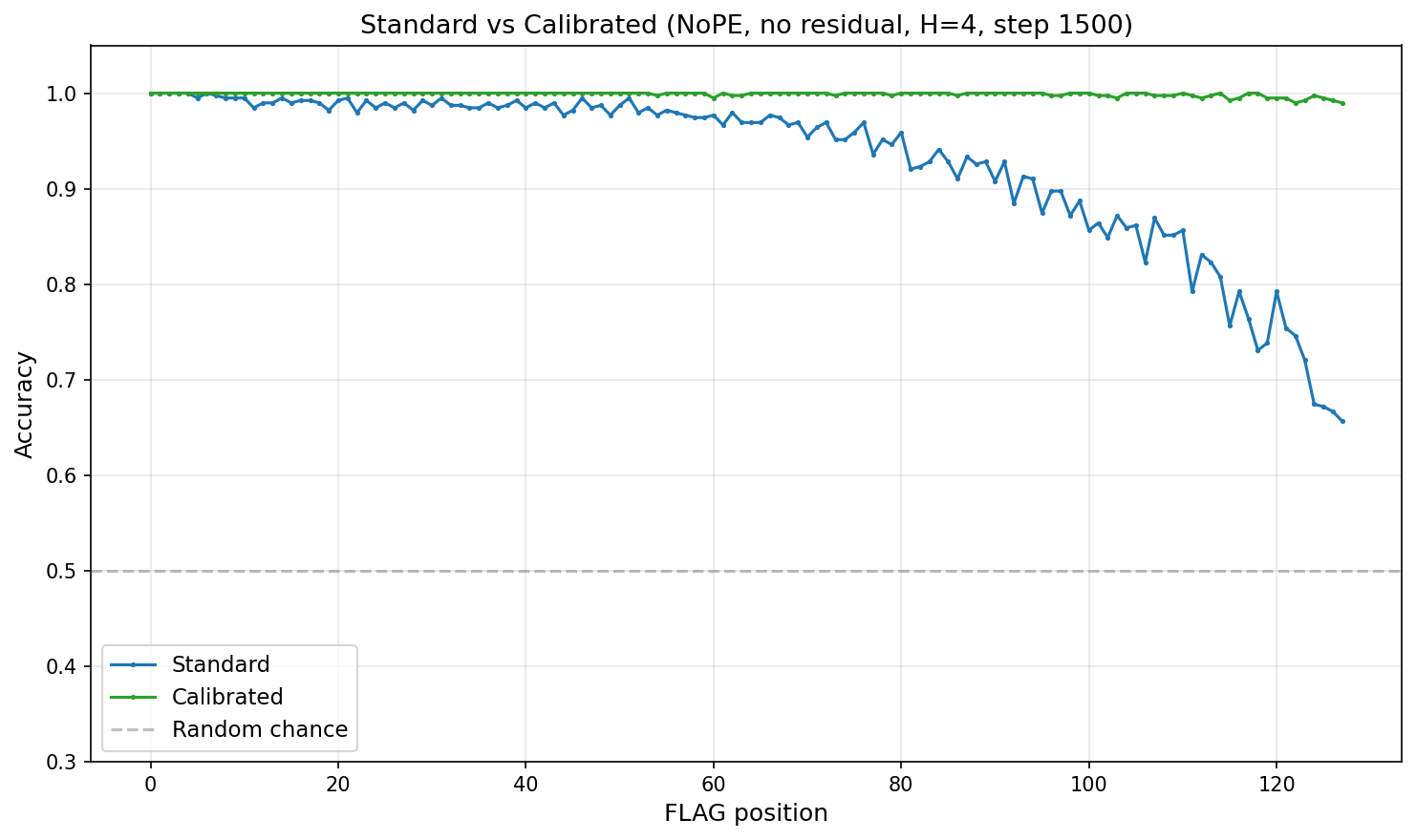
Success! I think this is about as much fun as I can have with this toy model, so I will stop here.

What are the takeaway lessons? I found it entertaining that this initially counter-intuitive behavior could be both understood — and corrected — so simply. To me it also seems to highlight that LLMs truly store information about the past very differently from humans.

Let us now discuss a wild analogy to physics. Consider a 1d rod of length L with a finite density of electric charge distributed uniformly on it. What is the energy of the rod? You can do a quick calculation and find that since each little bit of charge interacts with other little bit, the energy of the rod grows faster than L; this actually means that the system does not have a sensible thermodynamic limit as you take L huge, and all kinds of bad things4 can happen (e.g. very sensitive dependence on boundary conditions etc.).

In some sense the situation with the uncorrected transformer was very similar: every token talks to every other token, and thus bad things happen (e.g. very sensitive dependence on boundary conditions) when we try to take the thermodynamic limit of long sequences. This is related to the O(N^2) cost of running the attention mechanism itself. My fix above seems to have effectively solved this problem by diluting the magnitude of the contributions from earlier on, resulting in a system that now has a sensible thermodynamic limit. (In the physics analogy, we have found a way to screen the long-range Coulomb interaction). But one feels that the correct solution should have instead smoothly diluted the information content of the contributions from earlier on rather than simply reducing their magnitude. I don’t know how to do that5, but it feels like a fun and (possibly quite important) problem.