Should we be optimistic about Europe’s economy?

This morning, I saw a portfolio manager on Squawkbox Europe (CNBC). Or was he an analyst? In any case, he was very upbeat about the economy of Europe, which prompted me to comment.

What he especially referred to was the strengthening of the economic surprise index of the Eurozone, and he was correct. There has been a notable improvement in the “economic surprises” of late.

The spike is big, yes, but we should make some comparisons before celebrating. What you notice, for example, is an even bigger spike after the Russo-Ukrainian War collapse during the latter part of 2022.

The thing you should understand about the Citigroup Economic Surprise Index is that it is a weighted historical standard deviations of data surprises.1 What this means is that if the underlying data is very negative (note also that the index gives more weight to recent data), even small positive surprises can create major swings in the index to the upside. Moreover, the baseline is created by the median, or “consensus,” forecasts of each indicator in the Bloomberg economists-analyst survey. Therefore, if the consensus view is very negative, like when Europe is hit by a major energy shock(s), small upbeats in the actualized or “hard” data can create major spikes in the index.

We can assert, with a high certainty, that the jump we’re seeing in the Eurozone’s economic surprise index has been created by the murky view of analysts meeting some positive upside surprises in the realized economic data.

OECD’s leading indicators present a more concise picture. We updated the indicators of China, G-20 countries, Japan, four major European economies, and the U.S. until June in the Weekly Forecasts 27/2026.

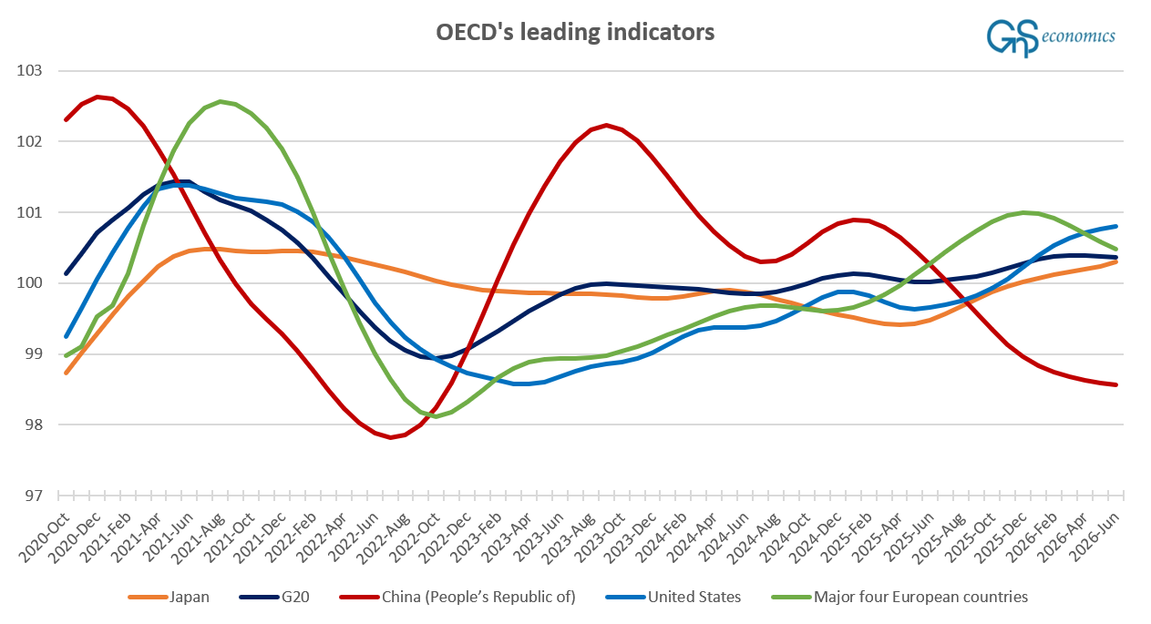
We summarized the message of the figure as

First, Figure 1 confirms that the downturn of the four major European countries (France, Germany, Italy, and the U.K.) has commenced. Secondly, it shows that the Chinese economy’s downturn has continued, but the decline has slowed in the past two to three months. This is indicative of an approaching increase in stimulus by Beijing and hence another upturn in the Chinese economy.

I will comment on the China stimulus in a later post, but the main message of the leading indicators is that the downturn of the European economy looks to have commenced in February. Leading indicators are also slow-moving, which means that they follow the underlying trends of the economies. What this implies is that they pick up the true momentum of the economy, not just the “surprises.” China appears to have been driving both the European and global business cycles during the past 16 years or so. Therefore, the conclusion we draw from the leading indicators is that the downturn of the European economy is likely to continue.

When we forecast where the European economy is heading in the short- to medium-terms, we should also consider this.

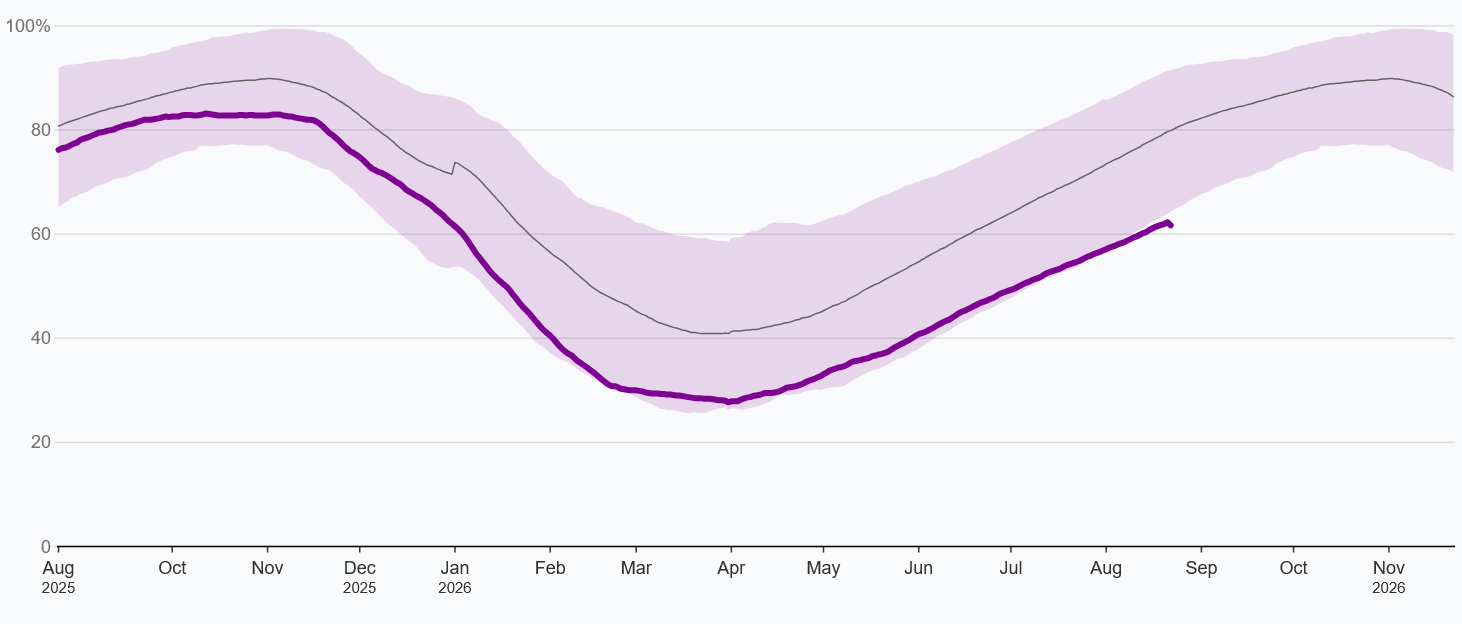
We are way below the five-year average and even below the five-year minimum in gas storage levels in the EU. Gas rationing is a real possibility this winter if the war in the Middle East re-escalates (which is likely) and if the winter is cold. Fortunately, due to the super El Niño, the winter is forecasted to be mild. Still, optimistic for the European economy, the above is not.

Have a cautious start for the week,

Tuomas

Share

The information contained herein is current as of the date of this entry. The information presented here is considered reliable, but its accuracy is not guaranteed. Changes may occur in the circumstances after the date of this entry, and the information contained in this post may not hold true in the future.

No information contained in this entry should be construed as investment advice nor advice on the safety of banks. Neither GnS Economics nor Tuomas Malinen can be held responsible for errors or omissions in the data presented. Readers should always consult their own personal financial or investment advisor before making any investment decision or decision about the banks in which they hold their money. Readers are solely responsible for the risks associated with using this post.

Readers must assess the risks and legal, tax, business, financial, or other consequences of their actions. GnS Economics and Tuomas Malinen cannot be held i) responsible for any decision taken, act, or omission or ii) liable for damages caused by such measures.