Rocket Science Slide Charts

The race between the United States and the Soviet Union to launch space craft into orbit around the earth, to the moon, and to the other planets in our solar system is generally agreed to have begun in 1955, with the announcement by the U.S. that they planned to launch satellites into space during the upcoming International Geophysical Year (July 1st, 1957 to December 31st, 1958). Five days after the U.S. announcement, the Soviet Union also announced that they planned to launch an artificial satellite “in the near future”, and the race was on.

The successes of the space race are well known, starting with the successful launch of the Sputnik 1 satellite by the Soviet Union in October 1957, cosmonaut and astronaut flights, space walks, communications satellites and spacecraft flights to the moon, Venus and Mars. With the Apollo manned Moon landings between 1969 to 1972, the race was effectively won. By the early 1970s budgets for space travel in the U.S. and the Soviet Union were considerably reduced and the space race was considered over.

Space travel requires many calculations to determine how to deliver a payload to a desired orbit or location in space, and how to keep it there once it has arrived. During the space race, many advancements were made in the field of digital computing that helped to speed up these calculations. However, the slide rule was still the only personal calculating device that most engineers and rocket scientists had immediate access to. While many space and rocketry calculations could be done using general purpose slide rules1, specialized slide rules for space-travel related calculations were also developed that allowed these calculations to be done more efficiently.

Probably the most famous space slide rule (among slide rule collectors at least) is the Aristo 80123 Martin Space Rule, from the early 1960s. Several articles have been written about this interesting rule in the Slide Rule Gazette2 and the Journal of the Oughtred Society3 among others4. However, it wasn’t the only space slide rule or slide calculator that was made. In this article, we’ll take a look at two slide calculators that were produced during the space race, each of which has specialized scales for computation of equations related to rocket design and space travel.

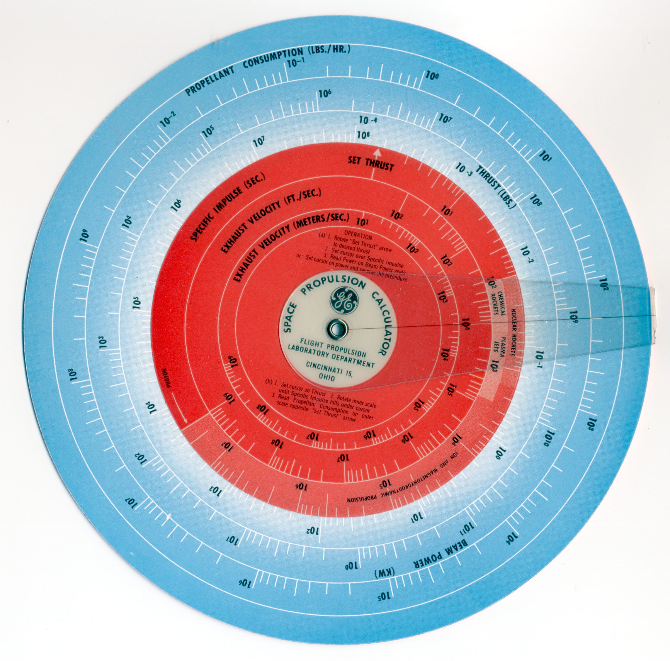
The General Electric (GE) Space Propulsion Calculator, introduced in 1958,5 was likely the first of the special purpose “Space Rules”. It is a 7-1/8” (18.1 cm) diameter two-sided circular slide rule/wheel chart made of thin plastic sheets, with scales and a cursor on both sides. Each side has a smaller circular disk that can be rotated relative to the larger base disk. The manufacturer of the calculator is not written on the calculator, but it has many of the characteristics of slide charts produced by Perrygraf, who produced many other slide charts and wheel charts for GE.

The front side of the calculator has scales for computations encountered in the design of rocket engines. These scales can be used to determine exhaust velocity, specific impulse, thrust, propellant consumption and beam power for chemical and nuclear rockets, plasma jets, photon rockets, ion drives and magneto-hydrodynamic propulsion systems. On this side, the background disk is colored with a light blue to white color gradient, and the rotating disk is colored red (see Figure 1).

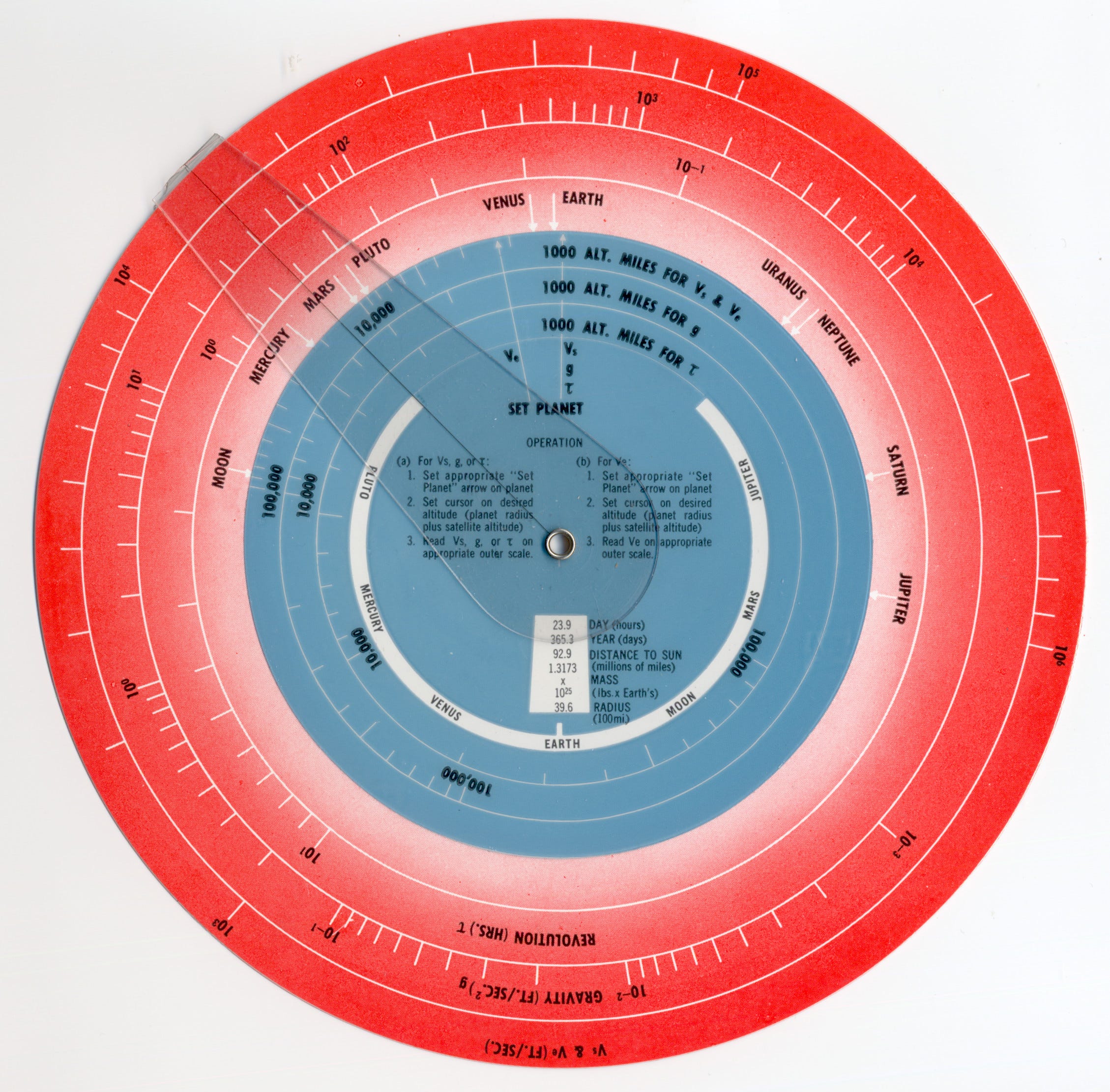
The reverse side of the calculator has scales that relate orbital altitudes with orbital periods, orbital velocity, escape velocities and gravitational forces for the Earth, the Moon and the other planets in the solar system. A cut-out in the central disk shows data for each planet, including the length of a day on the planet (in hours), the length of a year on the planet (in Earth days), the distance from the sun, the mass and the planet radius. The color scheme for this slide of the calculator is the reverse of the front side, with the background disk colored with a red to white color gradient, and the rotating disk colored blue (see Figure 2). The colors used on each side of the rule are particularly striking and eye-catching

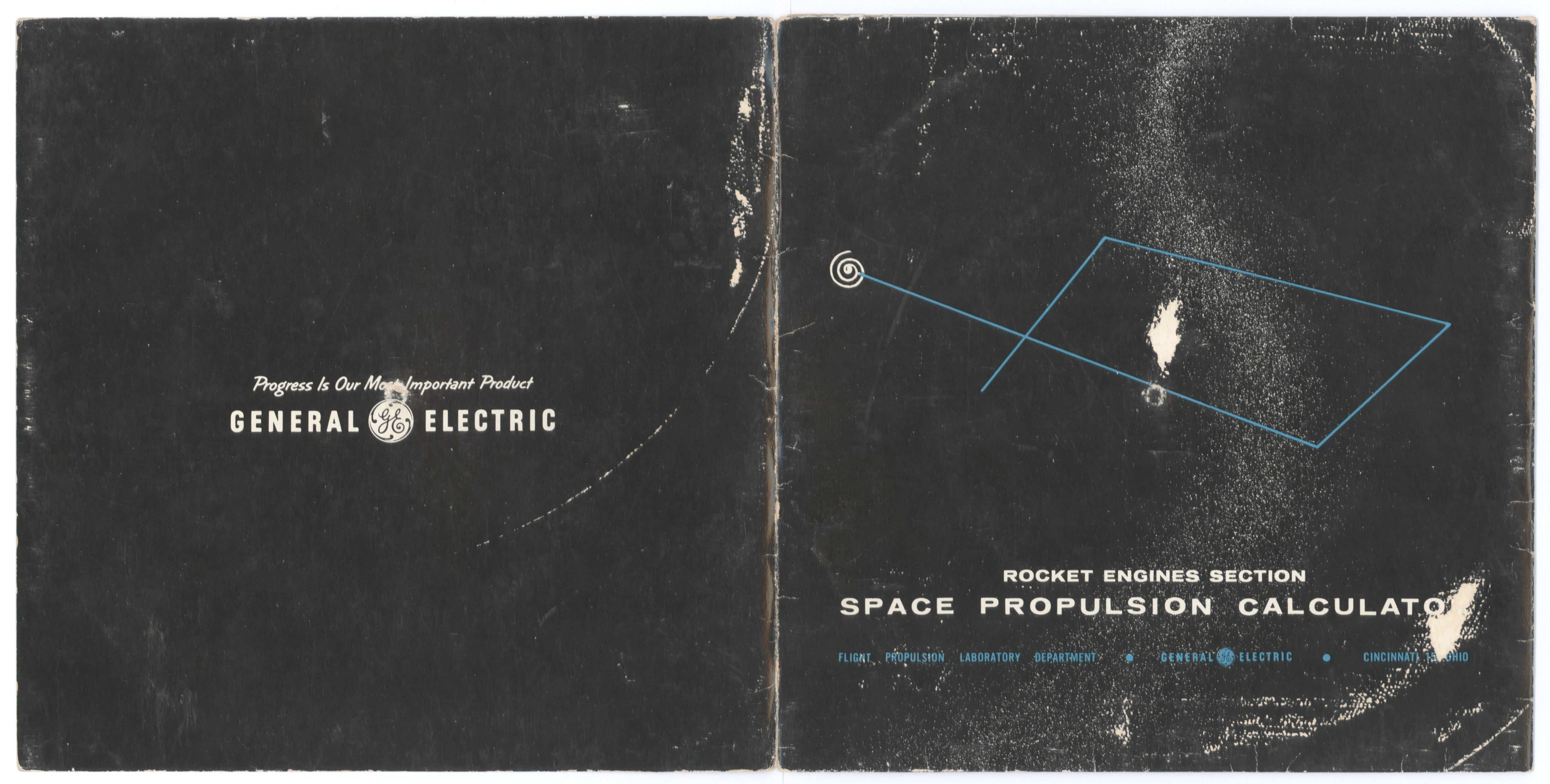
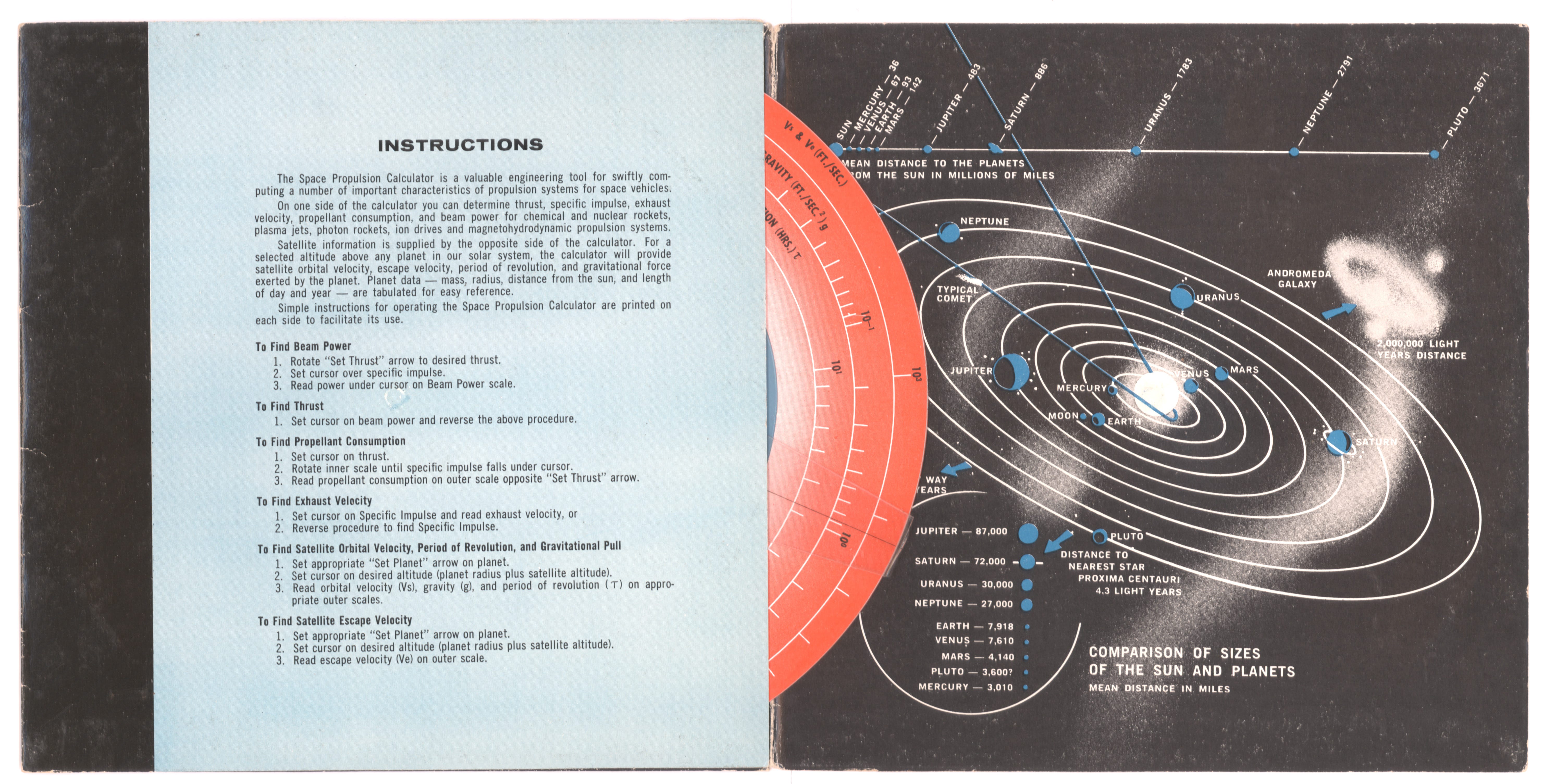
The calculator comes in a protective fold-out cardboard cover, with a pocket on the inside for the calculator. Operating instructions are provided in the inside of the sleeve, along with a picture providing data about the solar system planets. Basic instructions are also printed on each side of the calculator itself.

The instructions don’t provide the equations used by the calculator. However, they are quite well known and easy to figure out. All of the calculations on the front of the calculator incorporate a parameter used in rocketry called the specific impulse, I_SP. This is a measure of how efficiently a rocket creates thrust from a given amount of propellant. The unit of I_SP is seconds, and is the number of seconds for which 1 unit of fuel (e.g., 1 pound, kg or other unit of fuel) produces 1 unit of thrust (i.e., one pound, kg or other unit of thrust).6

Specific impulse (I_SP), exhaust velocity (v_e), thrust (F), propellant mass flow rate (m), power (P) and thruster efficiency (ŋ) are related to each other by the following set of equations:

where g₀ is the acceleration due to gravity on the Earth’s surface = 9.8 ms^-2. Thrust, exhaust velocity and propellant mass flow rate apply to all rocket types, while power and thruster efficiency are parameters used in calculations for ion, magneto-hydrodynamic or photon drive rockets.

The red disk on the front of the calculator has three scales. Two of the scales are for exhaust velocity, one graduated in meters/second from 10 m/sec to 10⁹ m/sec and the other in feet/second from 100 ft/sec to 10⁹ feet/sec. The third scale is for specific impulse ranging from 1 to 3×10⁷seconds. The specific impulse ranges for various types of rockets are indicated on the scale, including 100 to 400 seconds for chemical rockets (e.g., as used in launch vehicles that most people are familiar with), 400 to 2500 seconds for plasma jets (used for long-distance space travel), 2500 to 10⁵ and above for magnetohydrodynamic propulsion, and 3×10⁷ for photon rockets7.

The scales on the red disk can be used to compute the specific impulse given the exhaust velocity, or vice versa. Simply move the cursor to the known exhaust velocity or specific impulse, and read the corresponding value of the unknown parameter on the appropriate scale.

For example, in figure 1, the cursor is positioned at an exhaust velocity of 10,000 feet/second. The corresponding specific impulse is read as ~300 seconds (actual value = 310 seconds).

The Blue outer disk on the front of the calculator also has three scales, one for the propellant consumption in pounds/hour, one for Beam Power in kW, and the third for the thrust in pounds. The red inner disk also has a gauge mark/pointer labeled “SET THRUST” that used to set the thrust for a calculation, or read the computed thrust.

To calculate the thrust given the specific impulse and the propellant consumption, position the cursor at the propellant consumption in pounds/hour on the blue outer scale. Then rotate the inner red disk until the SET THRUST gauge mark is under the cursor. Next move the cursor to the specific impulse, and read the thrust under the cursor on the thrust scale.

For example, the Saturn V first stage booster had a specific impulse of 260 seconds and consumed ~30,000 pounds of fuel every second (15 tons of fuel per second!!!). What was the thrust generated? 30,000 pounds per second is equivalent to 1.08×10⁸ pounds per hour. First position the cursor at 1.08×10⁸ pounds/hour on the propellant consumption scale and move the SET THRUST gauge mark under the cursor. Next move the cursor to 260 seconds on the specific impulse scale, and read the thrust of 8×10⁶ (8,000,000) pounds on the thrust scale (actual value = 7,800,000 pounds) (see Figure 5).

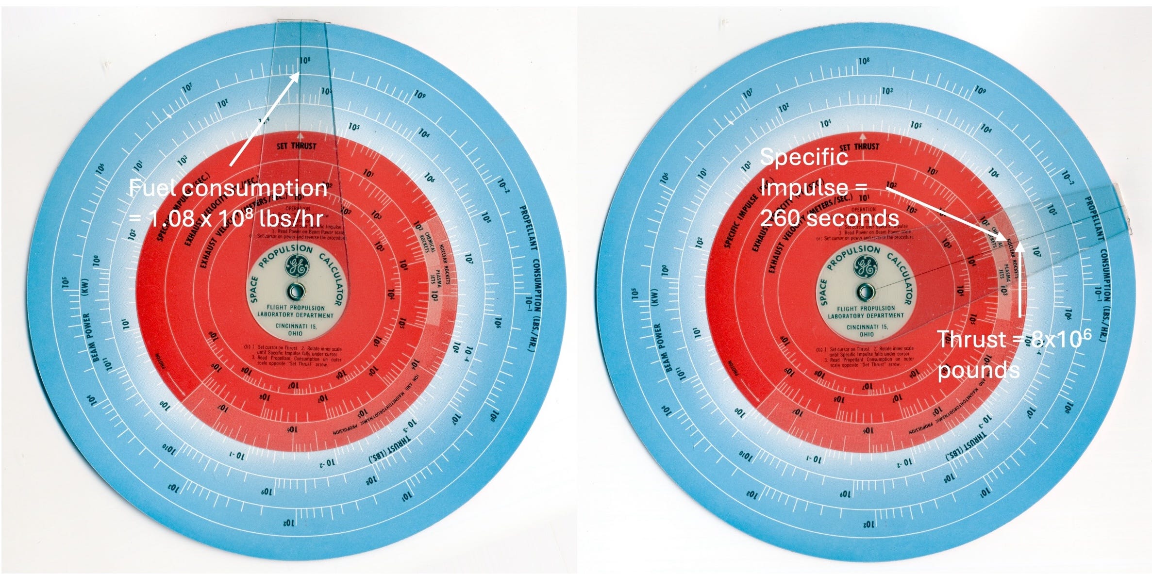
Given the power and specific impulse of an ion, electro-hydrodynamic or photon rocket, the thrust can be computed by positioning the cursor over the power on the beam power scale, rotating the inner disk until the specific impulse is under the cursor and reading the thrust on the thrust scale opposite the SET THRUST gauge mark.

For example, if an ion thruster has a beam power of 2.5kW and a specific impulse of 5,000 seconds, how much thrust does it generate?

Move the cursor to 2.5 on the Beam Power scale (units are in kW), then move 5,000 seconds on the Specific Impulse scale under the cursor. The thrust, 2.2×10^-2 (0.022) pounds force is read on the Thrust scale opposite the SET THRUST gauge mark. (See left hand side of Figure 6)

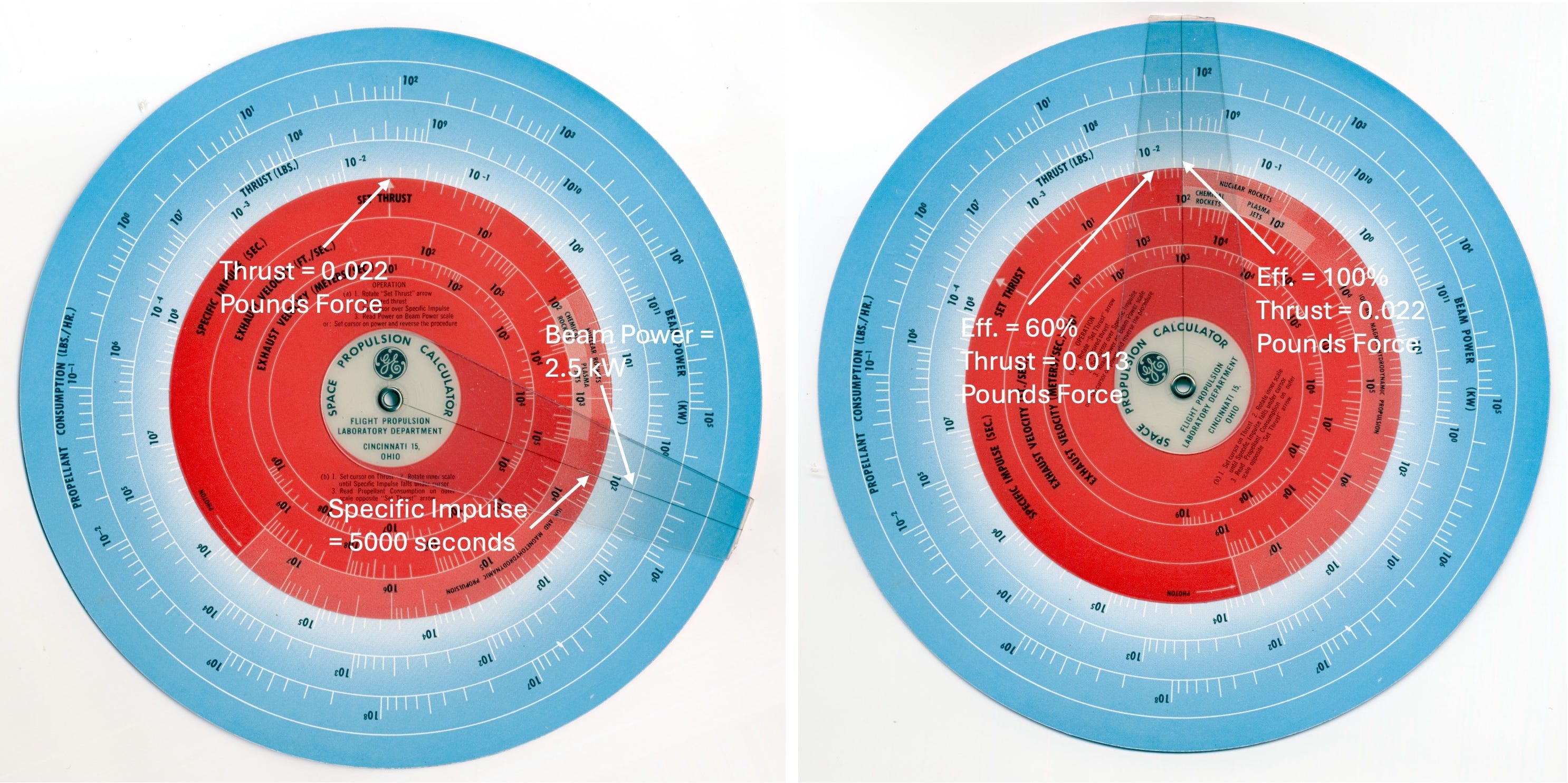
Note that the calculator doesn’t have a separate scale for thruster efficiency, ŋ. However, we find that the scales implicitly use a thruster efficiency ŋ=1.0 (i.e., 100% efficiency), as the answer computed above agrees with the result for ŋ=1.0.

If the efficiency is lower than 100%, then the corrected thrust can be computed on the calculator by moving the cursor to the SET THRUST gauge mark, then moving 10² on the Specific Impulse scale under the cursor. The corrected thrust is read on the Thrust scale opposite the efficiency value in percent on the Specific Impulse scale. For example, let’s assume an efficiency of 60% for the example above. When 10² on the Specific Impulse scale is moved under the cursor, we read the corrected thrust, 1.3×10^-2 (0.013) pounds force on the Thrust scale opposite 60 on the Specific Impulse scale, as shown in the right hand side of Figure 6.

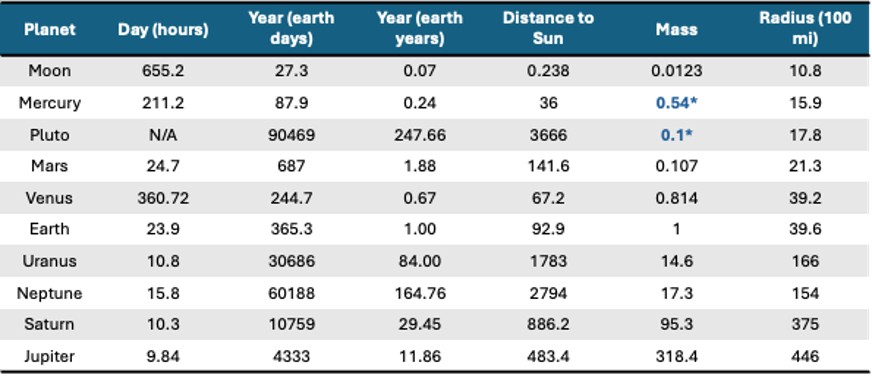
The scales on the reverse side of the calculator are used to compute the acceleration due to gravity (g) at a given orbital altitude (r), the time it takes a satellite to orbit a planet at that altitude (i.e., the orbital period, τ), the velocity at which the satellite travels (V_s), and the escape velocity (V_e) for that altitude.8 This data, sorted by planetary mass, is shown in the table below. Note, that here we use the expression planet to include the moon and Pluto, in addition to the actual planets.

In astrodynamics, the product of a planet’s mass, M and the gravitational constant G (= 6.67430×10^-11 m³kg^-1s^-2) is known as the standard gravitational parameter, µ. The equations for computing g, V_s, τ and V_e can be written in terms of µ and r as follows:

Clearly, the mass of the planet (which is used to compute µ) is an import parameter in all these equations. Comparing the masses given on the calculator in the window on the blue central disk and the current estimates of planetary masses, we see that the values on the calculator are quite close, except for a couple of cases that are highlighted in blue with an asterisk in the table above.

• The mass of Mercury is given as 0.54 Earth masses, while the correct value is 0.054 Earth masses. Since the radius of Mercury shown on the calculator is close to the actual radius, the value of 0.54 appears to be just a typo.

• The mass given for Pluto is 0.1 Earth masses, and its radius is given as 1,780 miles. This is similar to the size and mass of Mars. The current accepted value for the mass of Pluto is a lot lower, at 0.00218 Earth masses, or around 1/50 of the mass shown on the calculator. This is only 1/6 the mass of the Moon, which has a mass of 0.0123 Earth masses.
  By 1958 the size and mass of Pluto were largely determined from observations of perturbations in the orbit of Neptune. Errors in the estimate of the mass of Neptune resulted in an over-estimate of the mass of Pluto. It wasn’t until the discovery of Pluto’s moon Charon in 1978, that the size and mass of Pluto were more accurately determined.

The outer red disk on the reverse side of the calculator has gauge marks that correspond to the value µ for the moon and each of the planets in the solar system.

The gauge mark for Mercury corresponds to the correct planetary mass of 0.054 Earths, and not the incorrect mass of 0.54 Earths shown in the planet data window for Mercury.

The gauge mark for Pluto is a little to the right of the gauge mark for Mars. However, this is inconsistent with the masses given for Pluto (0.1 Earth masses) and Mars (0.107 Earth masses) in the data window. Since the mass given for Pluto is slightly less than the mass for Mars, the gauge mark for Pluto should have been placed a little to the left of the gauge mark for Mars. Instead, the placement of the mark for Pluto corresponds to a mass of 0.125 Earth masses. Of course, given what we now know about Pluto’s mass, the gauge mark for Pluto should actually be placed far to the left of the gauge mark for the Moon.

The red disk also has scales for the orbital period τ, in units of hours, the acceleration due to gravity g, in feet/second² and the orbital and escape velocity, V_s and V_e, in feet per second.

The scale for orbital period only has a range from 0.1 hours to 10 hours, which limits its applicability for many computations. This is strange, as there is plenty of room on the scale for two more decades of scales, which would make this a lot more useful. For example it’s not possible to calculate the orbital period of a satellite orbiting the Earth at a distance of 26,200 miles, which is the geo-synchronous orbit radius with an orbital period of 24 hours.

The blue disk has three altitude scales, one used when computing τ, one when computing g, and one when computing V_s and V_e. The disk has two gauge marks, one used for the τ, g and V_s computations, and the other for the V_e computations.

For orbital computations for a given planet, one of the two gauge marks on the blue disk are first positioned opposite the planet gauge marks on the outer red. The cursor is then positioned on the altitude scale on the blue disk corresponding to the desired parameter, τ, g or V (V_s or V_e), and the result is read on the corresponding scale on the outer red disk.

For an example of using the calculator for an orbital computation, we’ll compute the orbital period, gravitational pull, orbital velocity, and escape velocity for a satellite orbiting at an altitude of 5000 miles above the surface of the earth.

Since the earths radius is ~4000 miles, the altitude for this computation is 4000 + 5000 = 9000 miles. We start by positioning the τ, g, V_s gauge mark on the blue disk against the Earth gauge mark on the red disk. Moving the cursor to 9000 on the τ altitude scale on the blue disk, we read an orbital period of between 4 and 5 hours under the cursor on the orbital period scale on the red disk (maybe 4.7 hours - actual period is 4.786 hours). Some additional tick marks on the scale to indicate 1/10 or 1/6 of an hour would help improve the reading accuracy.

Next we move the cursor to 9000 miles on the gravitational altitude scale and read a gravitational pull of ~6.2 ft/sec² under the cursor on the Gravity scale on the red disk (actual value 6.23 ft/sec²). Moving the cursor to 9000 miles on the velocity scale, we read an an orbital velocity of ~1.7×10⁴ ft/sec on the velocity scale on the red disk (actual velocity is 17,250 ft/sec).

To compute the escape velocity, position the escape velocity gauge mark on the blue disk against the Earth gauge mark on the outer disk. Position the cursor at 9000 on the velocity altitude scale on the blue disk, and read an escape velocity of ~2.3×10⁴ ft/sec on the velocity scale on the red disk.

Longtime readers of Following The Rules may recognize the form of the orbital time equation from Mike’s earlier article Kepler a’la Bode. In that article we learned that the K and A scales could be used to easily compute relative orbital periods since the values on the scales are related by the formula K = A^3/2. This same relationship exists between the altitude scale for computing τ on the inner disk and the Revolution (Hrs.) τ scale on the outer disk. One decade of the altitude scale is 1.5 times longer than one decade of the τ scale9.

The Electrical Propulsion Calculator is a plastic coated cardboard slide chart calculator made by Perrygraf for Electro-Optical Systems, Inc., with a copyright date of 196710. The scales on the calculator allow users to quickly and efficiently perform computations related to electric propulsion systems. Electric propulsion systems use electricity generated by solar panels or nuclear reactors to accelerate ionized propellants to high velocities. Since the exhaust has such high velocity, electric propulsion systems are generally characterized as having high specific impulse (i.e., high efficiency), typically in the 1,000s. However, the relatively low power typically available for powering electric propulsion systems means that they usually have much lower thrust than chemical reaction powered rocket engines.

Electric propulsion systems are commonly used for in-space maneuvering, such as making steering corrections to satellites already in space, as well as for deep space missions. While the high specific impulse means that they are much more efficient than chemical propulsion systems, the low thrust makes them impractical for launch vehicle propulsion, where chemical rockets dominate.

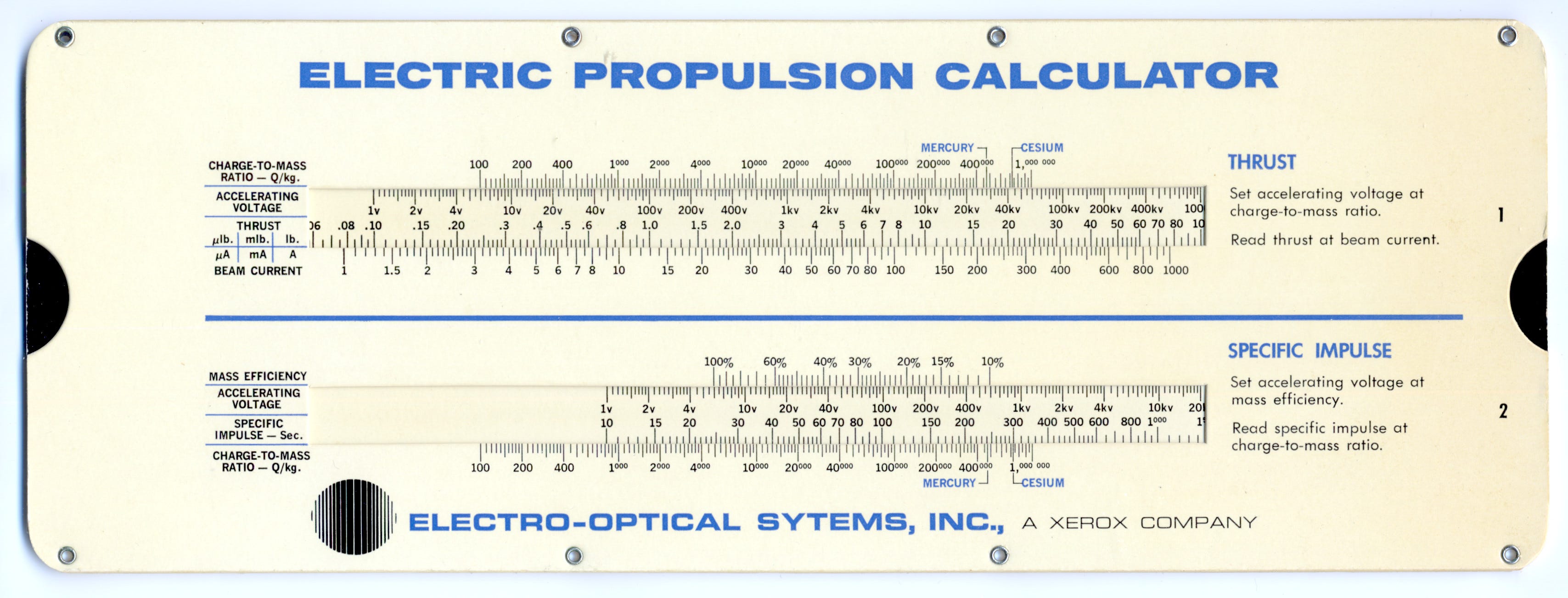
The scales on the front of the calculator allow users to compute the thrust and specific impulse of electric propulsion systems, given the accelerating voltage, beam current and charge to mass ratio of the particles being accelerated.

The scales on the reverse side enable users to compute the required propellant weight and power needed given the duration in days for which the propulsion system will need to be fired.

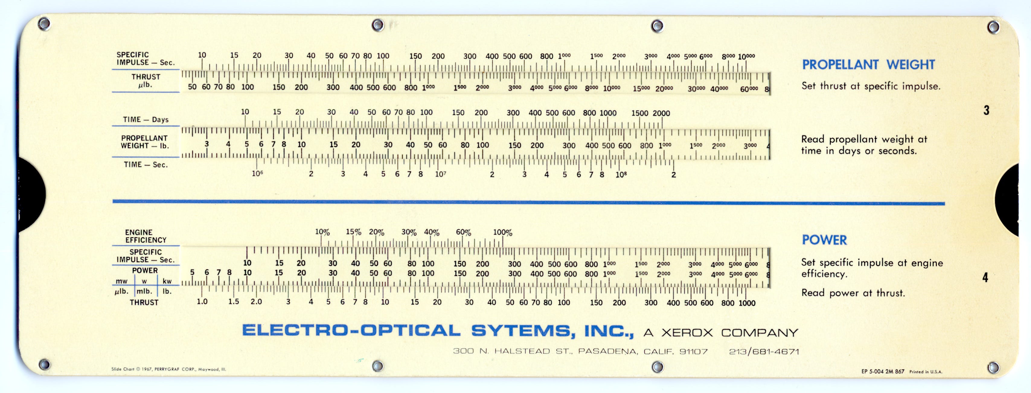
The calculator comes in a plastic sleeve that provides instructions on how to use the calculator, and also shows the equations implemented by the calculator. Several of the equations that the calculator computes are similar to those on the GE Space Propulsion Calculator, but there are additional scales for calculations specific to Electric Propulsion systems.

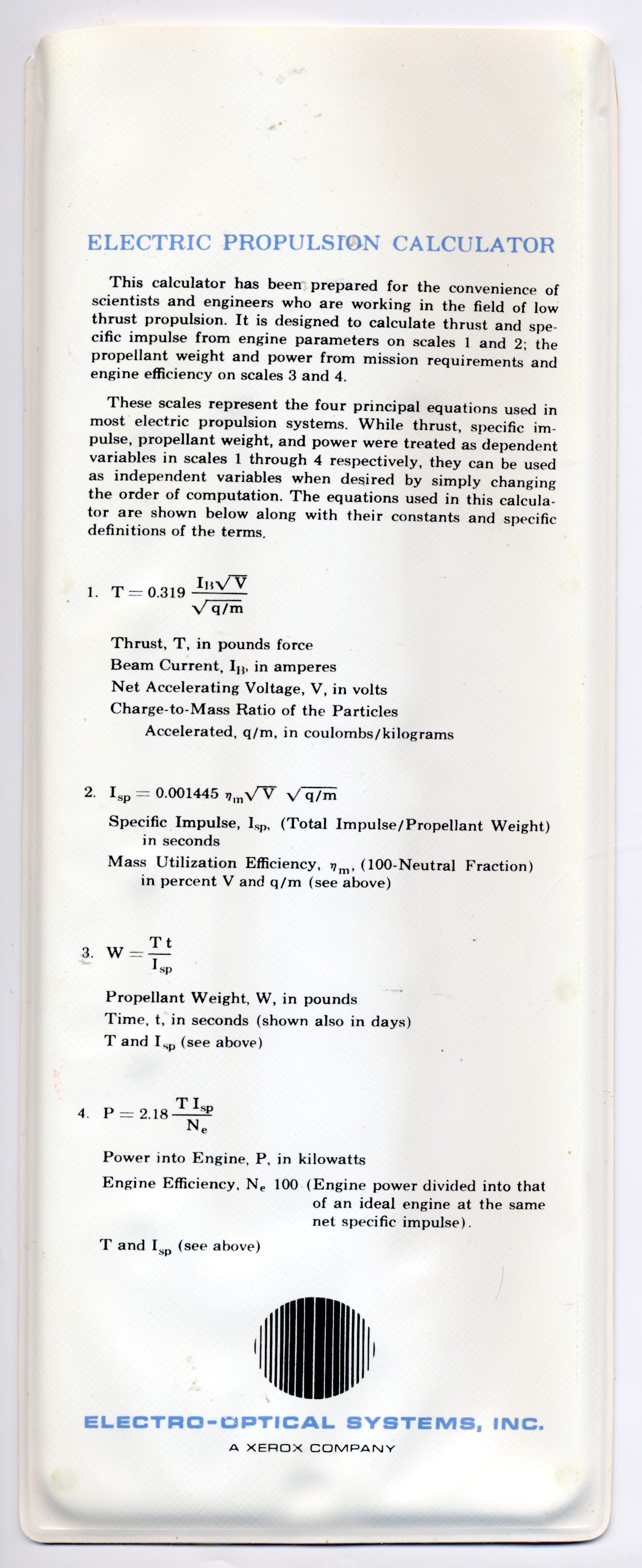
The instructions include a reminder that while the scales each have one parameter treated as a dependent variable, they can be treated as independent variables by changing the order of the computations. This is a powerful feature that is inherent to all slide calculators.

Let’s take a look at the equations governing the thrust generated by an electrical propulsion system. We start with the basic thrust equation for any rocket engine, i.e., thrust is the product of the mass flow rate ṁ, and the exhaust velocity, v_e:

When an ion with mass m and electrical charge q is accelerated by an electrical potential difference (i.e., the voltage V) to a speed v_e, an amount of electrical potential energy given by the product qV is converted to kinetic energy given by the equation qV = ½mv_e². By combining these equations, we can derive a formula for the exhaust velocity, as follows:

The quantity (q/m) is known as the charge to mass ratio for that ion.

The beam current I_B is the total electrical current carried by the accelerated ions as they leave the thruster. It equals the product of the mass flow rate ṁ (i.e., propellant mass consumed per unit time), and the charge to mass ratio, i.e., I_B = ṁ(q/m). Rearranging, we can express the mass flow rate in terms of I_B and (q/m) as follows:

Substituting the expressions for v_e and ṁ into the thrust equation above, we obtain an expression for the thrust of an electrical propulsion system in terms of I_B, V_B and (q/m), as follows:

We note that the usable power P consumed by the electrical propulsion system is the product of V and I_B, i.e., P = VI_B. Of course, if there are any inefficiencies, then the actual power consumed by the system will be higher.

Recall that the specific impulse is given by the equation I_SP = v_e / g₀. Substituting the expression for v_e above into this equation gives us an equation for I_SP in terms of the accelerating voltage V and the charge to mass ratio (q/m) as follows:

There are four groups of scales on the calculator, numbered 1 to 4. The first group of scales relate the thrust T in pounds to the ion beam current I_B in amps, the accelerating voltage V in volts, and the charge to mass ratio q/m in columbs/kg. The equation given on the sleeve for these scales is:

This is the similar to the equation shown in the Electric Propulsion System Equations section, but with a scaling factor of 0.319 to express the thrust in pounds instead of newtons. Sine 1 newton = 0.2248 pound force, the scale factor = √2 × 0.2248 = 0.319.

The charge to mass ratio scale has gauge marks for mercury (at 482,000 coulombs/kg) and cadmium (at 727,000 coulombs/kg). These materials were among the first propellants used in ion-thruster systems in the 1960s11. Modern electric propulsion systems use inert noble gases such as xenon (easy to ionize, but expensive), krypton or argon (cheap), although many other propellants have also been experimented with.

The second group of scales compute the specific impulse I_SP in seconds given the accelerating voltage V in volts, the charge to mass ratio (q/m) in coulombs/kg, and the mass efficiency factor η_m as follows:

Comparing this equation with the equation for I_B in the Electric Propulsion System Equations section, we find that the constant 0.001445 = (1/100) × √2 / g₀. Notably, the mass efficiency η_m in the equation on the sleeve is treated as a value between 0 and 100, and not a value between 0% and 100% (i.e., between 0 and 1).

The third group of scales give the weight12 of propellant W in pounds required to fire a thruster for a given amount of time t in seconds, when given the thrust T in pounds, and the specific impulse I_SP in seconds. The formula is:

The thrust scale on the calculator for this equation is graduated in µ-lbs (millionths of a pound). There are also two time scales on the calculator, one graduated in seconds, and the other graduated in the equivalent number of days.

The fourth set of scales relate the beam power, thrust, specific impulse, and engine efficiency N_e. The power scale can be read in units of mW, W or kW opposite thrust units of µlb (micro-pouns), mlb (milli-pounds) or pounds force, which nicely extends the range of values handled by the calculator.

The equation implemented by these scales is given as:

where P is in kW, T is in pounds and N_e as a value between 0 and 100.

We have previously seen a variant of the equation in our discussion of the GE Space Propulsion Calculator, i.e, I_SP = (2N_eP) / (Tg₀).13 Rearranging this, we have P = (g₀/2)(TI_SP / N_e). Since 1 pound = 4.448 newtons, and g₀ = 9.8ms^-2, we see that the constant 2.18 in the Electric Propulsion Calculator comes from (9.8 / 2) × 4.448 × (100 / 1000).

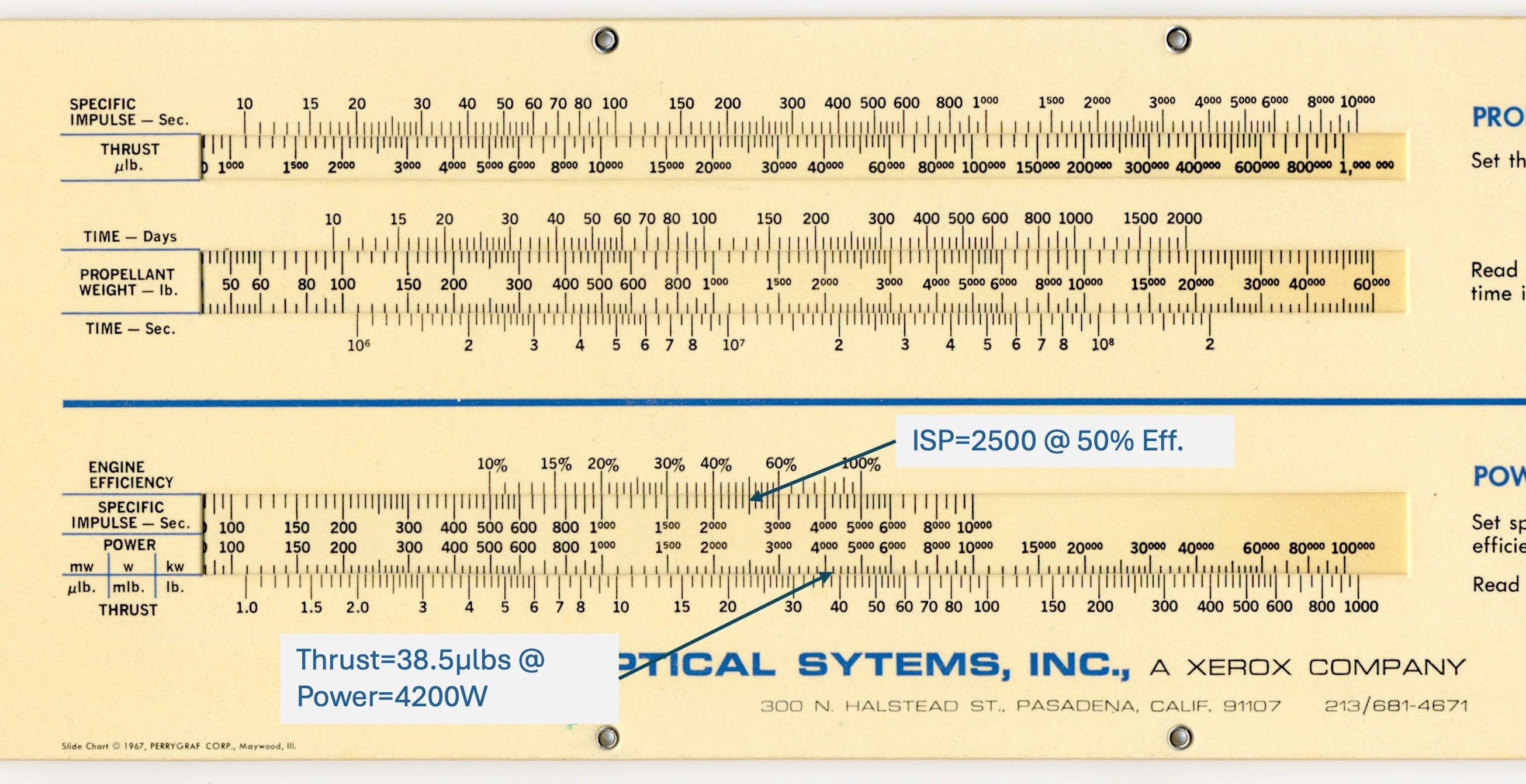
For a real-world example of electric propulsion system calculations, we shall use the SpaceX Mini Argon Hall Effect Thruster used in the SpaceX Starlink V2 Mini satellites. This operates with a power of 4.2kW, a specific impulse of 2,500 seconds and 50% total efficiency.

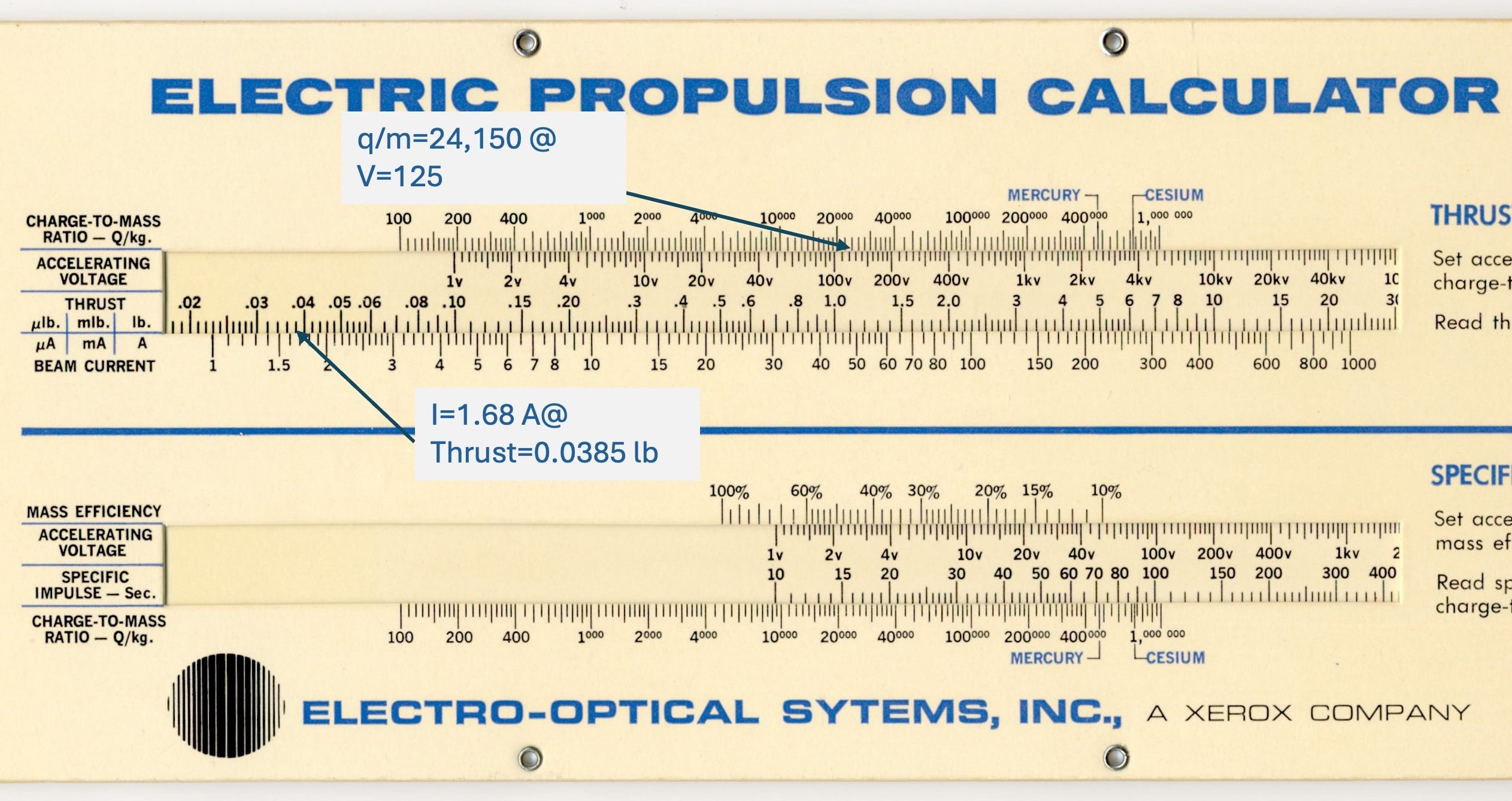
First, let’s compute the thrust of this engine. Using scale group 4, position 2,500 on the specific impulse scale opposite the 50% efficiency mark. Opposite 4,200 watts on the power scale, read a thrust of 38.5 mlbs (0.0385 pounds force).

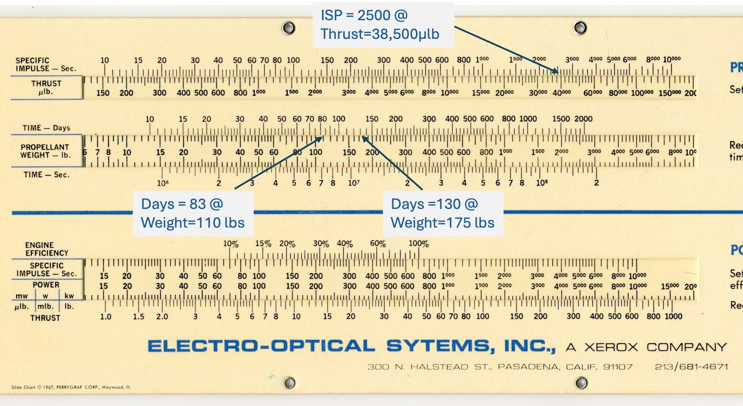
While SpaceX hasn’t published the mass of Argon in their satellites, it is estimated by aerospace analysts to be between 110 and 175 pounds. How many days of continuous engine burn does this translate to?

Using scale group 3, position 38,500 µlbs on the thrust scale opposite 2,500 seconds on the specific impulse scale. Opposite 110 on the propellant weight scale, read 83 days. Opposite 175 on the propellant mass scale, read 130 days.

What is the accelerating voltage and beam current used in the SpaceX engine?

We can compute these values by first using scale group 2 to compute the accelerating voltage V. We could then compute the beam current as I_B = η_mP / V, but we will also see how I_B can be computed using scale group 1.

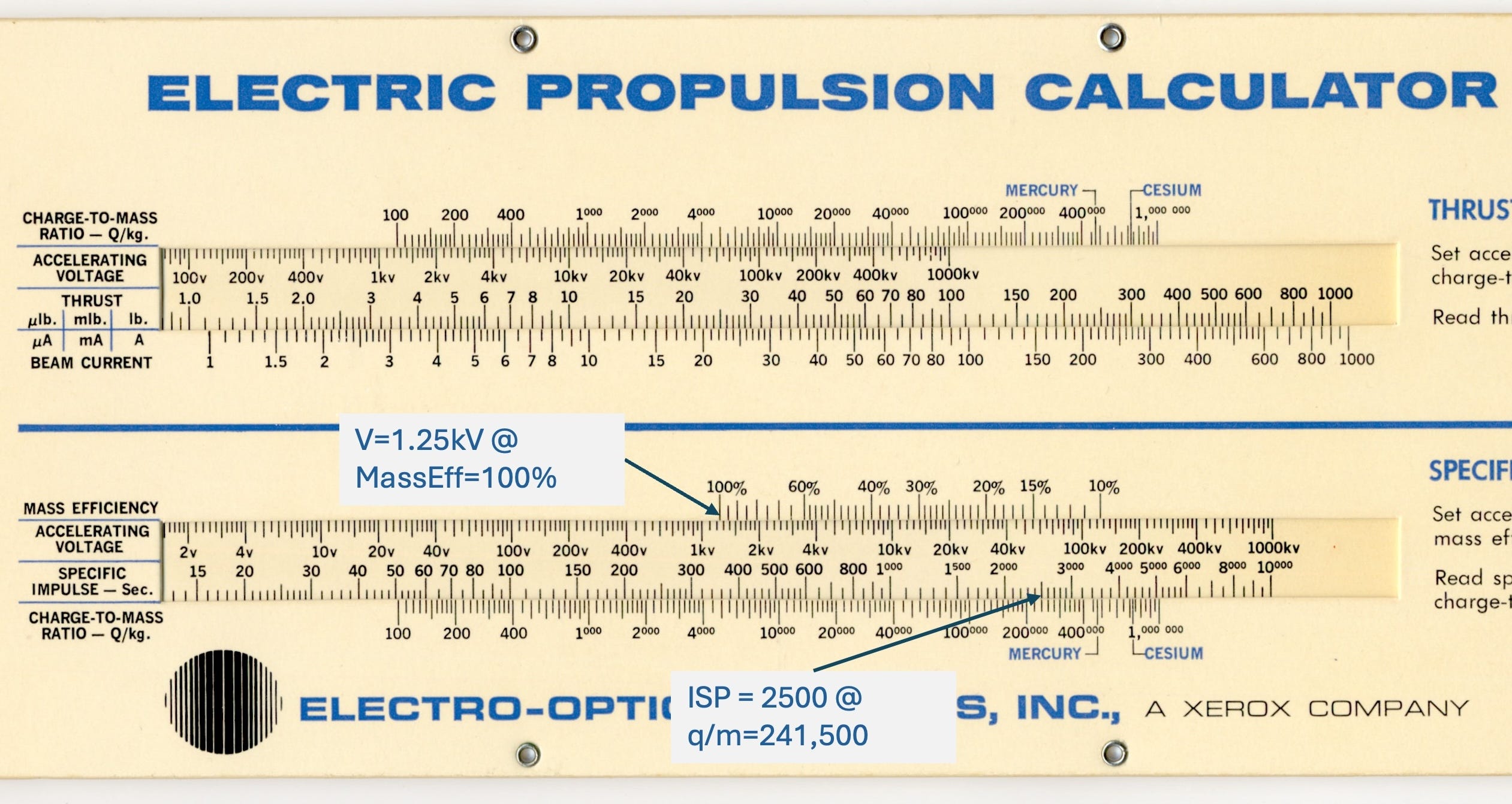
Argon has a charge to mass ratio of 2,415,000. This poses a slight problem, because the charge to mass ratio scales on the calculator only extend to 1,000,000. No worries - we can work around this by computing the voltage for a charge to mass ratio of 241,500, and dividing the result by 10. For this exercise, we keep things simple and assume a mass efficiency of 100%, although in practice, a mass efficiency of between 85% and 90% is more likely.

Using scale group 2, position 2500 on the specific impulse scale opposite 241,500 on the charge to mass ratio scale. Opposite 100% on the mass efficiency scale, read 1.25kV on the accelerating voltage scale. Divide this by 10 to get the desired accelerating voltage of 125 volts.

Using the formula I_B = Pη_m / V, we have I_B = 4200 × 50% / 125 = 16.8 A

We can also compute I_B using scale group 1. Once again, the charge to mass ratio scale doesn’t extend beyond 1,000,000, which is less than the charge to mass ratio for Argon. In this case, we will compute the beam current required for a charge to mass ratio of 2,415,000 / 100 = 24,150. We then multiply the calculated beam current by 10 to get the desired beam current. Position 125V on the accelerating voltage scale opposite 24,150 on the charge to mass ratio scale. Opposite 0.0385 on the thrust scale, read a beam current of 1.68 A. Multiply this by 10 to get the beam current of ~16.8 A.

The GE Space Propulsion Calculator and the Electro-Optical Systems Electric Propulsion Calculator are two of just a handful of slide rules and slide charts ever made with scales for rocket science calculations. The GE calculator can solve basic rocketry and orbital equations, while the Electro-Optical calculator is even more specialized, with scales focusing on ion propulsion computations.

Of the two, the Electro-Optical calculator is easier to use. It’s scales are arranged to perform computations with just one setting of the slide, while computations on the GE calculator usually require multiple steps. Accuracy is also much better on the Electro-Optical calculator, as the tick marks on the scales are much closer together than on the GE calculator. The scale ranges on the Electro-Optical calculator also appear to be more appropriate for engineering calculations.

Both calculators have their period-specific quirks. The planetary data for Pluto on the GE calculator is very outdated, and the value given for Pluto’s mass is now known to be in error by a factor of 50(!). And of course the International Astronomers Union (IAU) no longer classifies Pluto as a planet (although many astronomers still disagree with this). The Electro-Optical calculator has gauge marks for the two propellants used in ion propulsion systems at the time. The range of values on the charge-to-mass scales didn’t anticipate the future use of Argon as a propellant, although we saw that it is possible to work around this restriction.

With large gaps between scale tick marks and and the needlessly restrictive ranges on one or two scales, it’s not entirely clear who the target audience was for the GE calculator. It falls slightly short of being a serious engineering tool, although it’s still very useful for producing quick estimates for many space related computations. The Electro-Optical calculator is more of a high-end engineering calculator. At the time of its introduction, chemical rockets were the norm, with just a few experimental ion thrusters having been flown into space. As we saw, the calculator is fully capable of handling calculations for modern ion propulsion systems. The only improvement would be to extend the charge to mass ratio scales to handle higher q/m propellants in use today.

Both calculators are just really, really cool to use. It’s pretty amazing to see how a couple of pieces of cardboard sliding against each other can be used to quickly solve rocket science calculations.

Speaking of which …

Also, this post is going out on July 4th 2026, so Happy 250th birthday celebrations to our U.S. readers!