Markout Standard Errors

I recently published data on liquidity provider (LP) performance using variable cost ratios, which is the expense/revenue ratio. Below are some statistics that are not in that paper. The LP expense consists of the estimated LP theta from the negative gamma of constant-product automated market makers (AMMs), while the revenue is from fees. Fees are easy to estimate, but theta is not, which is why AMM protocols can justify ignoring LP expense altogether, and promote APYs of 50%+ on their homepages (“it’s ambiguous!”).

Perhaps the best way to measure LP theta is high-frequency markouts. These mark each swap transaction’s fill price—including fees—with a Binance/Coinbase price in 12 seconds ahead. Summing these PnLs generates a net PnL for the day, which, when subtracted from the fees, generates the theta expense. The problem is that creating years of second-downsampled databases is a pain. Once created, merging second-downsampled data with swap data is time- and effort-intensive, as large datasets are rife with errors that need to be identified and corrected.

Here, I compare the 12-second markout LP variable cost ratio with two alternatives. One is to use the end-of-hour CEX price data, which contains only 24 datapoints each day, instead of 86400 for a second-downsampled dataset. A swap at 8:01 AM or 8:59 AM is marked against the 9:00 AM CEX price. The other markout uses an end-of-day CEX price for all the swaps that day.

The total-sample theta/fees estimates are virtually identical across these three approaches, with pools ranging from 24 to 64 months of data. Over shorter horizons, the higher-frequency markouts have much lower variability because there is less time for random movements to generate noise. The question is: how long does it take for the simpler hourly and daily estimates to reach the 12-second markout efficiency?

To estimate the standard errors, I used the bootstrap approach. The bootstrap estimates a standard error by mimicking repeated sampling from the data-generating process using the data itself. You repeatedly resample daily data, recompute the statistic of interest each time, and take the standard deviation of those recomputed statistics. That standard deviation approximates the statistic’s true sampling variability—its standard error—because the empirical distribution of resampled statistics stands in for the unknown sampling distribution.

I used consecutive days in each bootstrap estimate because variance is autocorrelated, and variance is a primary driver of the LP’s expense. Consecutive-day resampling preserves autocorrelation, and the standard deviation of the resampled n-day ratios estimates the standard error of the n-day ratio estimator.

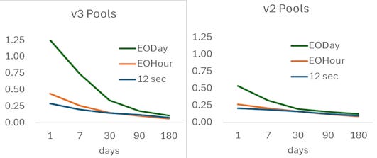
There is virtually zero difference in the standard errors between the 12-second and hourly markout estimates after 30 days for v3 pools. For the v2 pools, the difference is trivial at 1 day and identical at 7 days. End-of-day markouts are fine for v2 pools applied for 30 or more days, while for v3 pools, it takes about 3 months for the EOD markout to approximate the efficiency of the hourly and 12-second markouts.

A major issue in EOD markout PnLs is the effect of anomalous swaps that are really LP trades. These are when an LP comes in with 10, 100, or 1000 times the pool’s liquidity and either applies it to a single trade or for a few minutes or even an hour. These transactions do not affect true LPs, as they are clearly a targeted attempt to generate a position rather than capture fees, and they can result in outliers that are patently absurd. Thus, one can apply a few common-sense rules to remove these transactions, such as eliminating the swaps that started or ended with liquidity more than 10 times the daily median liquidity.

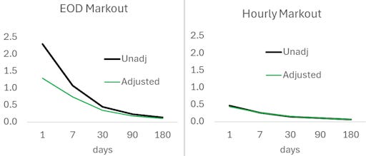
I only did this with v3 pools, because these shenanigans do not occur with v2 pools. Below, we see that the EOD markout standard errors are significantly affected by these anomalous swap transactions in the short run. However, after 30 or perhaps 90 days, the impact of these swaps effectively diversifies away. Most interestingly, these crazy transactions do not affect the end-of-hour markout estimates, regardless of the targeted sample window. The implication is that if you are using hourly CEX markouts, you do not have to filter out the anomalous swaps. If you are estimating LP performance over a year, it probably won’t matter even if you are using a simple EOD markout.

Finally, there is the option of using hourly markouts vs. using the AMM’s price 250 swaps ahead. For relatively liquid pools that trade over 1000 times a day, this is anywhere from 1 to 6 hours ahead. The advantage of the 250+ approach is that one does not need to maintain a CEX database; instead, one can use a pool’s swap event logs. Below, we see that after 90 days, the hourly CEX and internal 250+ markout estimates have comparable efficiency.

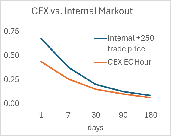
In sum, v2 pools are easy-peasy, so using a daily markout is all benefit and no cost. For v3 pools, end-of-hour markouts are just as effective as 12-second markouts applied for a month or longer, and they eliminate the need to filter for anomalous-liquidity swaps. If you are looking at many pools with many coins, and do not have hourly CEX data, you can use the AMM’s own prices taken from event logs, and after 90 days, the standard error for a theta/fee ratio will be around 0.1, which is close to its minimum of about 0.05 for this metric.