
This article is the second of my series Statistics with Python. In Part 1 I looked at built-in Python functions and the statistics module. Now I will show how many of these statistics are calculated as this is more enlightening than using a “black box” function. Several of these statistics require iterating over the entire dataset so the code in this article, which calculates a raft of stats with just a single iteration, might be faster than calling several builtins. This is a hypothesis I will investigate in Part 3.
I don’t want to mix up the discussion of the various statistics we will be calculating with the discussion of the actual code, so will run through it first. If you understand this stuff already just skip straight to Coding
The statistics we’ll calculate are the following:
Count
Total
Arithmetic Mean
Minimum
Lower Quartile
Median
Upper Quartile
Maximum
Range
Inter-Quartile Range
Standard Deviation of Population
Standard Deviation of Sample
Variance of Population
Variance of Sample
Skew
Many of these are self-explanatory but a few might not be familiar so I will give a brief overview of those.
I am sure everyone understands the arithmetic mean: it is what most people think of as the “average” and is just the total of all numbers divided by the count. It is one of several values known as “measures of central tendency” which are intended to give an idea of a central or typical value. However, if the data is not evenly distributed this can give a distorted impression, so the median gives a better idea of a typical or central value. It is quite simply the middle value when the data is sorted into order.
The quartiles are examples of percentiles, ie. the values a certain percentage from the beginning and end of sorted data. Lower and upper quartiles are the values 25% and 75% along respectively. Their purpose is to complement or even replace the minimum and maximum values which might be what are known as “outliers”, ie. they are significantly lower or higher than the main body of values and therefore give a misleading impression of the range. I have used the terms lower quartile, median and upper quartile, but the terms 1st, 2nd and 3rd quartile are also widely used. Quartiles are probably the most widely used percentiles but any percentage can be used, deciles (the 10th and 90th percentiles) also being commonly used.
Calculating quartiles and the median sounds simple, just make sure the data is sorted and pick the relevant values from it. However, it’s not quite so simple because if there is an even number of values in the data there is no single middle value. In this case we take the mean of the two central values. Irrespective of whether the count is odd or even, the counts of the lower and upper halves may be odd or even, requiring the same approach as with calculating the median.
In order to show how the quartiles and median are calculated in each of the four possible permutations, I will show some sample data.
Firstly, the overall count is odd, but the count of the two halves used to calculate the quartiles is even. The blue cells show the quartiles or the cells averaged to calculate the quartiles. The green cells are the median or cells averaged to calculate the median. Note that if the count is odd we ignore the median when calculating the quartiles.
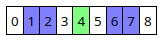
Secondly, the overall count is odd, but this time the count of the two halves used to calculate the quartiles is also odd so we just pick the middle values for the quartiles.
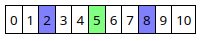
Next, the count is even and the count of the two halves used to calculate the quartiles is also even. The two median values are included in the values used to calculate the quartiles.

Lastly, the count is even but the count of the two halves used to calculate the quartiles is odd.
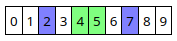
Measures of central tendency give no impression of how widely the data is spread so we will also calculate the range (maximum - minimum) and the inter-quartile range. The latter of course is useful in eliminating the misleading effects of any outliers. Such values are known as measures of spread and another is the standard deviation which deserves a section to itself.
The standard deviation can be thought of as the average (ie. mean) amount by which values differ from the mean. That is not a precise definition but it gives an impression of what it signifies. Of course the actual mean by which values differ from the mean would be 0 as positive and negative values cancel out. To get round this the variance is calculated using the squares of each value, and the square root is taken to obtain the standard deviation.
The standard deviation is a useful indicator in its own right but along with the variance it is also used to calculate other statistics such as various coefficients of skewness, as we shall see later, as well as in correlations and regressions and many other applications.
If you want a detailed description of standard deviation take a look at the Wikipedia article.
Another statistic we will calculate is a coefficient of skewness. I say a rather than the as there are plenty to choose from, the one I am using is Pearson’s second skewness coefficient (median skewness). Again you might like to read the Wikipedia article for full details but briefly this gives an indicator of how assymetric the data is around the median.
This project consists of a class called CalcStats with properties for each of the statistics and a method to calculate them. There is also a short program to test our class. These are the source code files which you can find in the GitHub repository..
calcstats.py
calcstatsdemo.py
I’ll now examine the code in calcstats.py a piece at a time. There are eleven sections but don’t let that put you off - most are pretty simple.
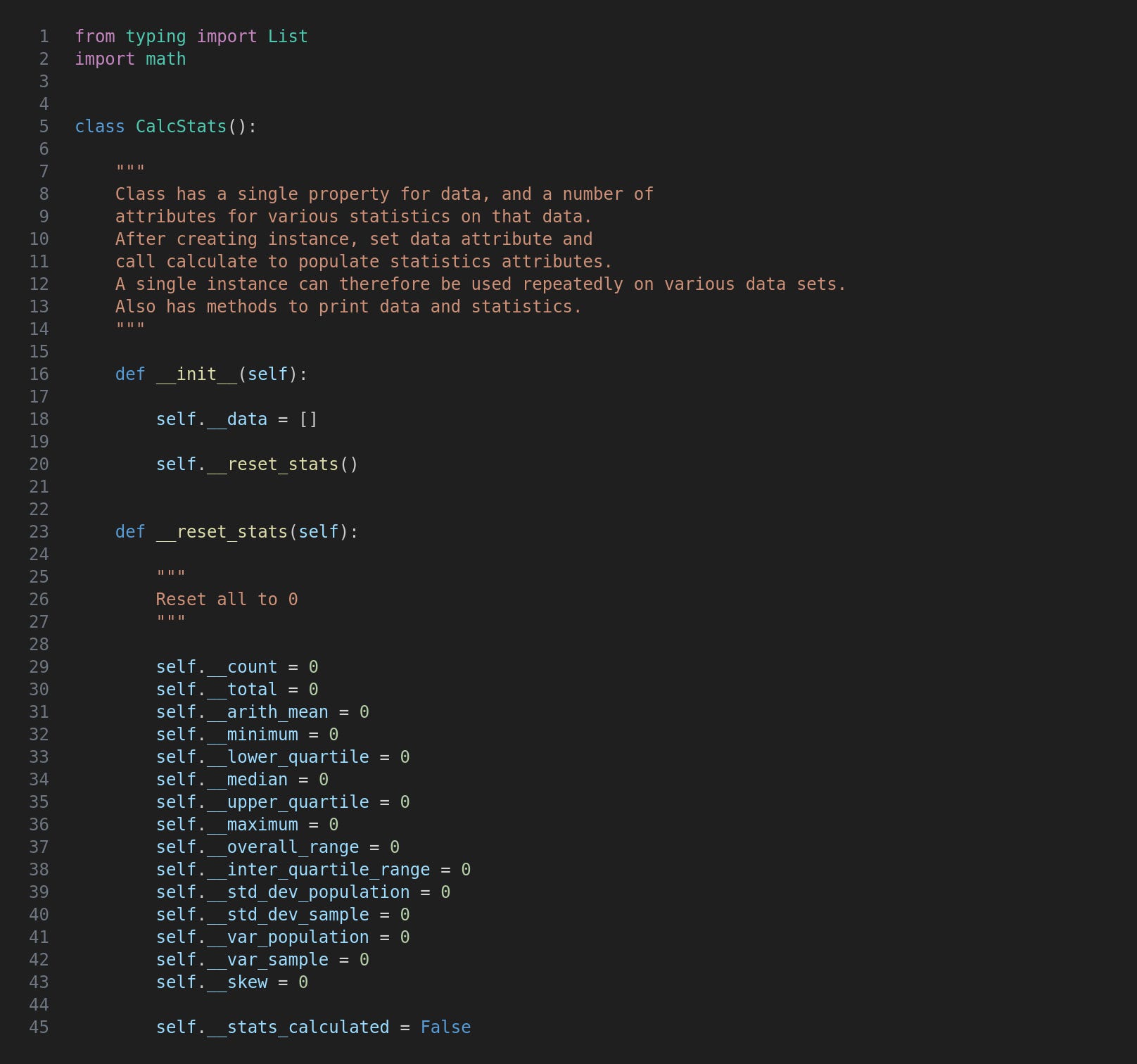
In __init__ a backing variable is created for data and initialised to an empty list, and __reset_stats is called. This function creates or resets all the backing variables to 0 depending on whether the class is being reused. The __stats_calculated variable is set to False for future use.
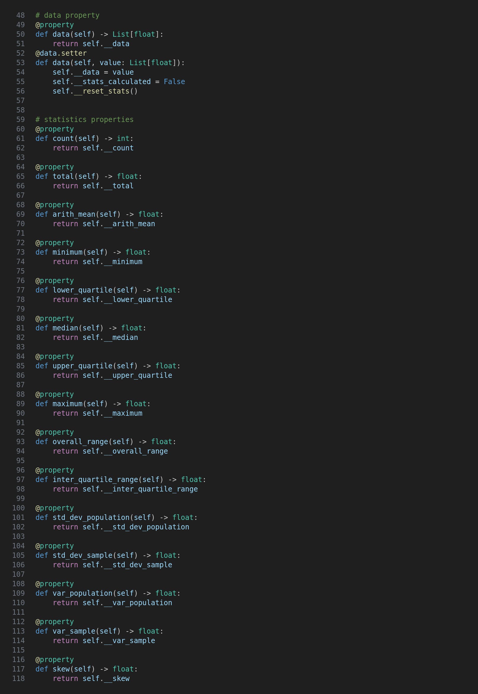
The first property is data and in its setter, as well as setting the backing variable, we also reset the statistics and set __stats_calculated to false. The rest of the properties are get-only so simply return the relevant variable.
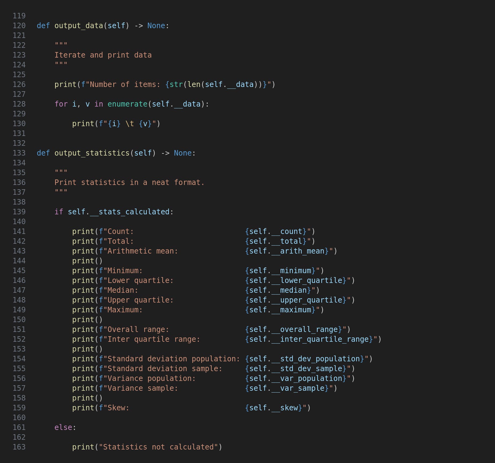
The output_data method prints the number of values in the dataset and then iterates the data, printing each row number and value.
In output_statistics the name of each statistic and its value are printed in a neat format although of course calling code can access each property for whatever purpose.

The age old problem of figuring out whether a number is even or odd. Why doesn’t the math module implement this? Anyway, I have used the classis mod 2 method but also included the and 1 method - if a number is odd its 1 bit will be 1, otherwise it is 0.
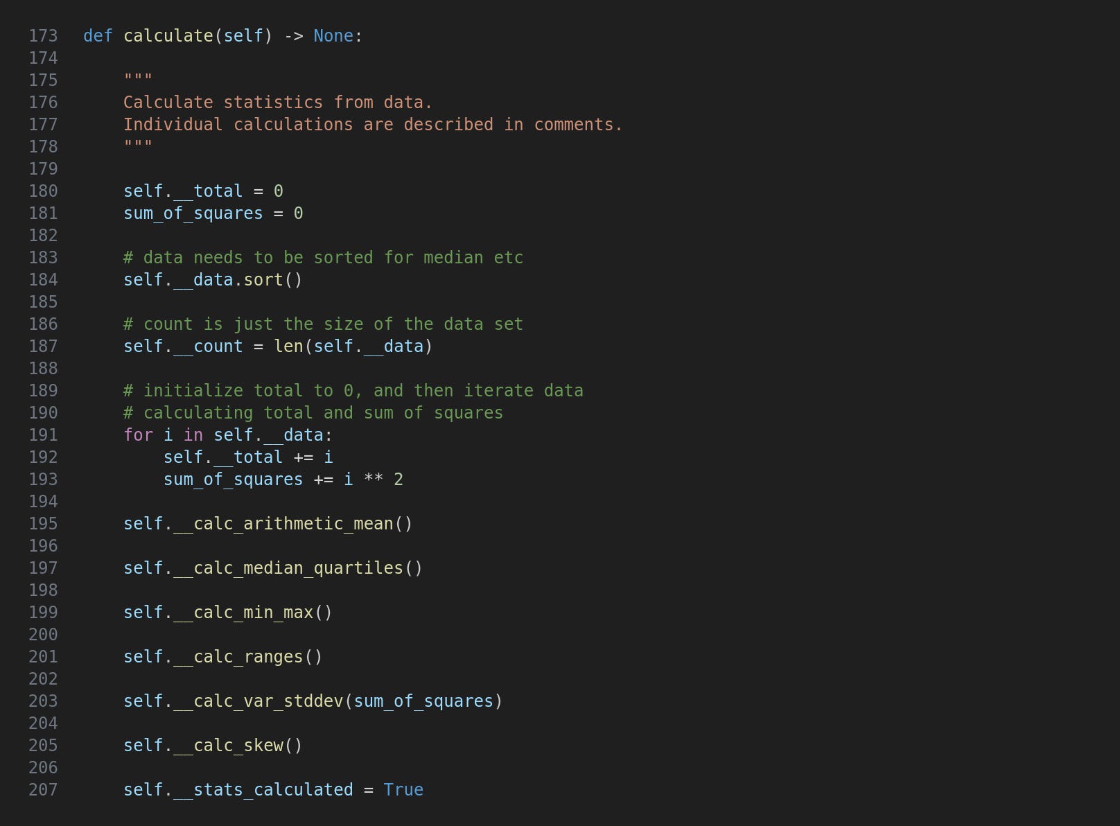
Most of the calculations live in their own separate functions which are called in calculate. Before that we set __total to 0 and create a variable for the sum of squares, sort the data and grab the length of the data. Then the data is iterated to build up the total and sum of squares. This is the single iteration I mentioned earlier and these variables are used in later functions, hence my hypothesis that this class is faster than several functions which each need to carry out their own iteration. Finally the __stats_calculated flag is set to True.

Nothing complicated here, we just divide the total by the count.
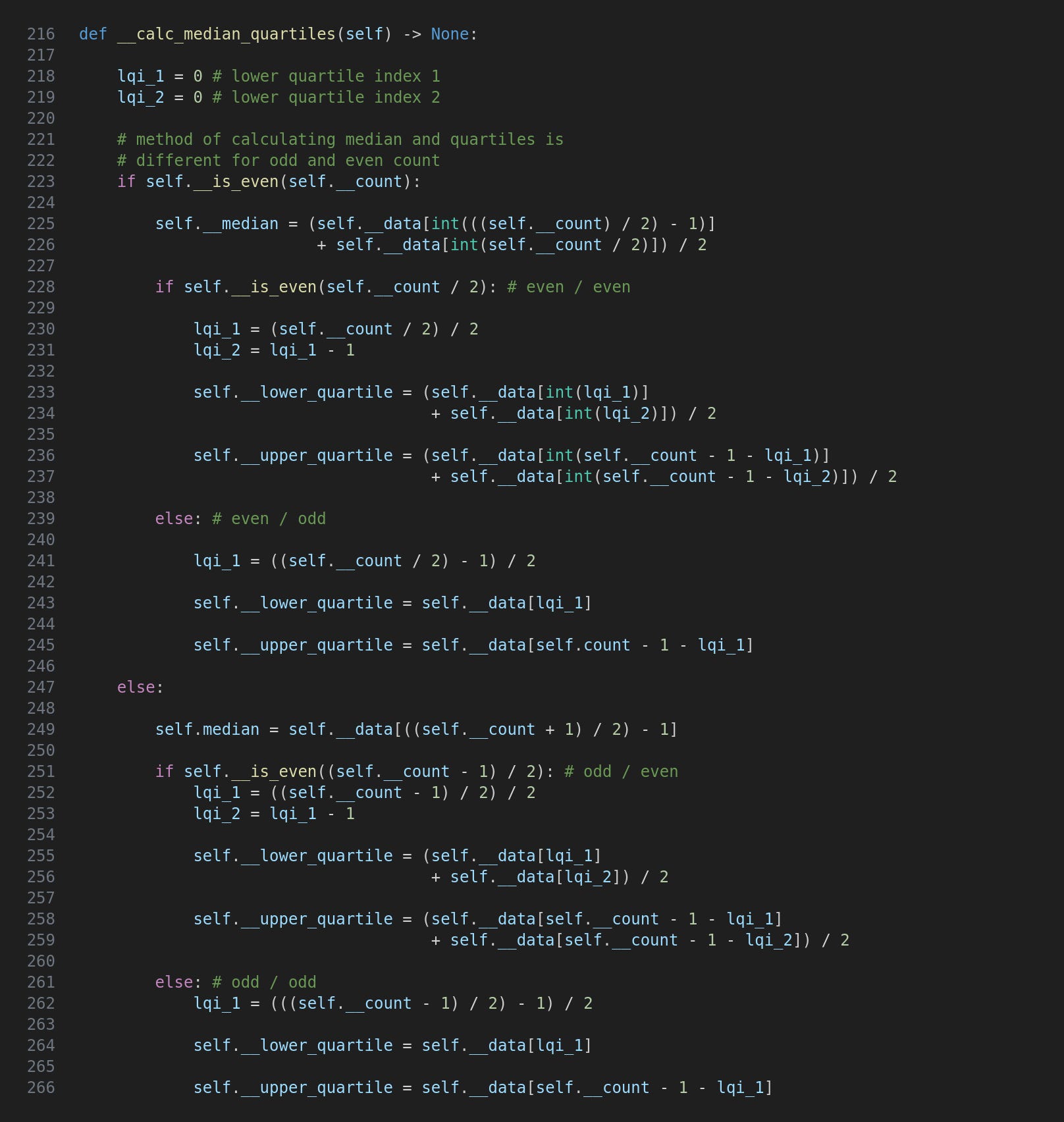
This function isn’t as complicated as it looks but is a rather tedious implementation of the process described above, allowing for various combinations of odd and even counts. Remember that for odd counts we use the middle value and for even counts the mean of the two middle values.

In calculate the data is sorted so the minimum and maximum values are the first and last respectively.

There are two ranges to calculate, the overall between the minimum and maximum, and the interquartile range between the quartiles. In each case these are just a subtractions.
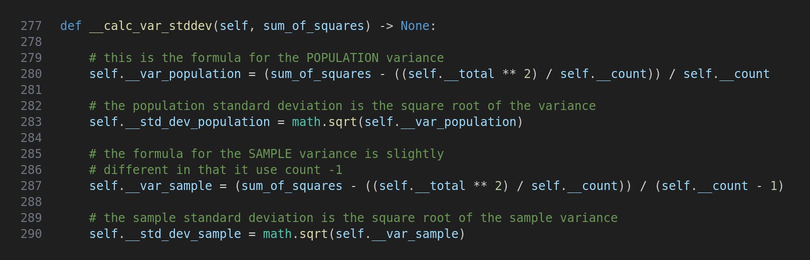
I am planning a separate article on variances and standard deviations so I won’t go into detail here. Note that there are two methods of calculating the variance depending on whether the data is a population (all data) or a sample (some of the data). As the standard deviation is the square root of the variance this also comes in two flavours.

This also is a topic which deserves its own article but note that it is a measure of how much the values are “squashed” towards either end. If the coefficient is positive the data is right-skewed and if it is negative it is left-skewed.
Now we can move on to calcstatsdemo.py where we put our code to use.
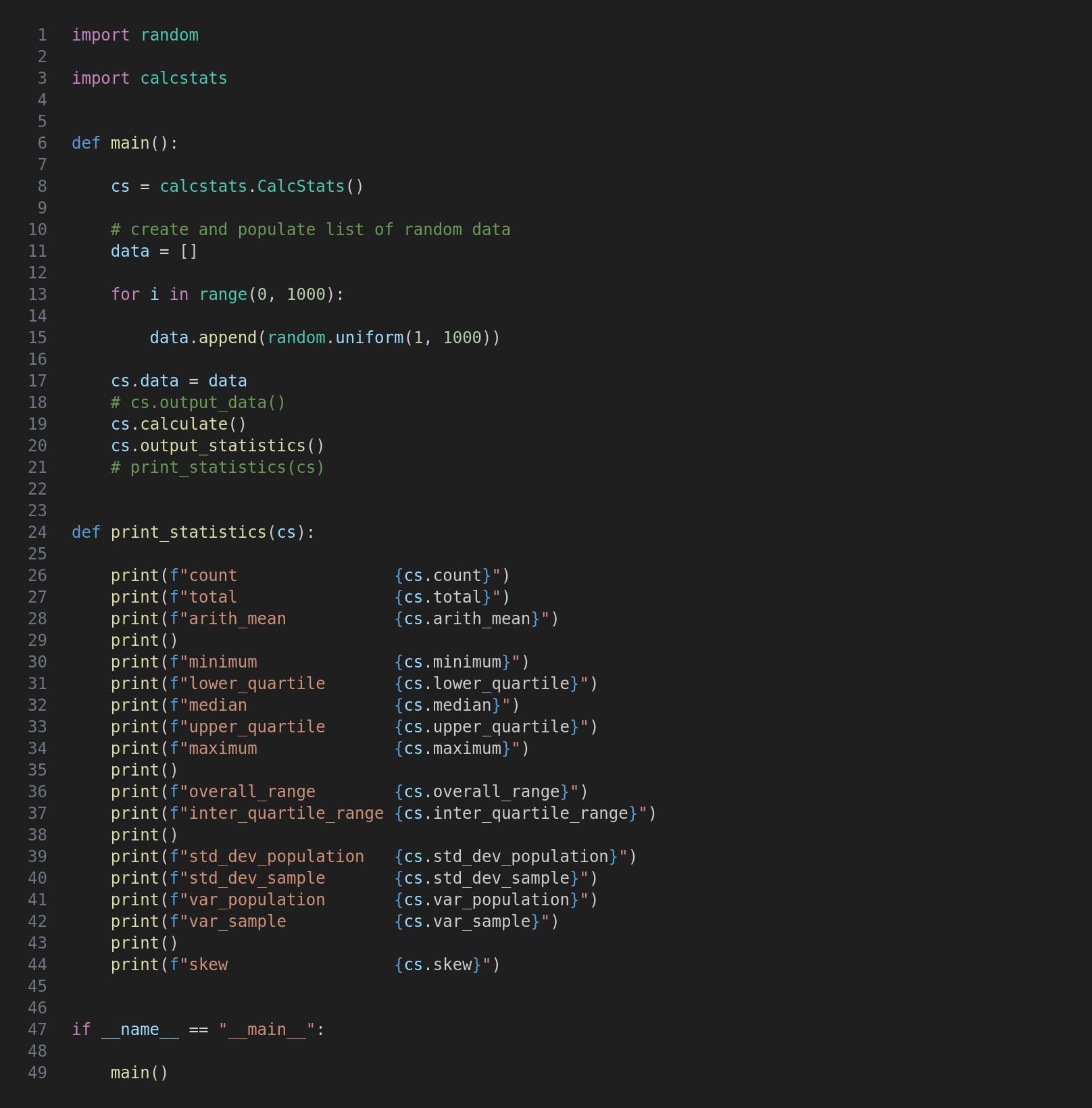
Firstly a CalcStats object is created and then a list for data. Random numbers are added to the list which is then set as the CalcStats object’s data. Then all we need to do is call the calculate and output_statistics methods.
You can uncomment the output_data() call if you wish, and I have also included a function to print the statistics although this only replicates the output_statistics method and is intended mainly as a reference for the property names.
Run the program with this command...
python3 calcstatsdemo.py
...which will give you something like this...
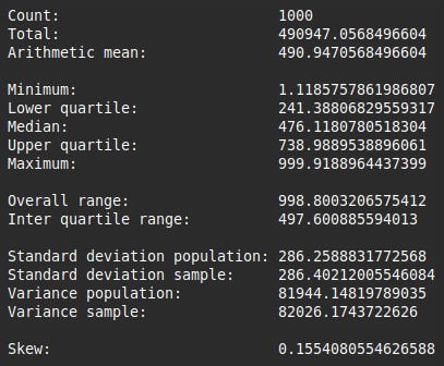
The sample data is created with random.uniform so the statistics all sit roughly where you would expect them to. The mean is around half way between the minimum and maximum. The median also is in about the middle of the range. The quartiles are about one quarter and three quarters of the way along the range. The skew is a very small value. Most real world data doesn’t follow this pattern!
In Part 3 I will run some tests to see whether the CalcStats class is faster than calling several built-in and statistics module functions.
For updates and random ramblings please follow me on Bluesky.
No AI was used in creating the code, text or images in this article.
Comments
Nothing yet. Say the first thing.
Sign in to join the conversation.