Geometric Algebra from Linear Algebra

This is Chapter 6 in Knowledge Graphs as Geometry, a weekly series developing a single thesis: every knowledge graph relation is an operation in space, and the dozens of named embedding models are one operation in different notation. The earlier posts selected a number system for each model by hand. This post derives the single construction that contains all of them, starting from the dot product alone. The executed code accompanies the post at the end.

Consider the models introduced so far. DistMult places entities in ordinary real space ℝ. ComplEx and RotatE move to the complex numbers ℂ, because a complex number rotates the plane. QuatE moves again to the quaternions ℍ, because quaternions rotate in higher dimensions and, unlike complex numbers, do not commute, which is what let QuatE represent ordered relation compositions that RotatE could not. Each step up this ladder supplied a new geometric capability, and each step was a choice made by hand. In every case we selected the number system that already contained the rotation we wanted.

These recurrences invite an explanation. It is worth asking why ℂ rotates the plane, why the quaternions rotate space, and why they fail to commute exactly when ordered composition is required. These are not separate coincidences. They are one object viewed at different sizes, produced by a single construction that yields ℝ, ℂ, ℍ, rotations in any dimension and their noncommutativity from one rule. The construction is the geometric algebra, and it is built from a single familiar operation, the dot product.

This post therefore asks what multiplication ties the family of models together and where it comes from. The position maintained throughout the series is that geometric algebra is the design language. It explains why ℂ and ℍ are the appropriate carriers and what a rotation is. Linear algebra is the implementation, since every product below is a plain tensor contraction in PyTorch with no special-purpose algebra engine. The algebra explains, and the matrices compute.

Vectors already support several operations. We add them, scale them and take their dot product. What is missing is a product of two vectors that returns an object we can continue to multiply. The dot product a·b returns a number, so it leaves the space of vectors immediately. The cross product exists only in three dimensions and is not associative. Neither operation lets us write a chain such as abc and reason about it as we reason about numbers.

We therefore require a product ab that is associative and ask what form it must take. Without yet knowing the product, we can split it into two parts, in the same way that any matrix splits into a symmetric and a skew-symmetric part:

The symmetric part measures how aligned the two vectors are, and the antisymmetric part measures how much they differ in direction. The single decision that defines the subject is to require the symmetric part to equal the dot product. That is the one rule:

Setting a = b gives aa = a·a = ‖a‖². In this algebra a vector squares to its own squared length, so the multiplication encodes distance. This single consequence is what allows a geometric algebra to express lengths and angles using products alone.

The antisymmetric part is a new kind of object. It changes sign when a and b are swapped, so it cannot be a scalar, because a single number that also carries an orientation exists only in special dimensions. It requires a new object. The dot product a·b records the line the two vectors share when they point in the same direction. The antisymmetric part records the plane they span when they point in different directions, together with the area that plane sweeps and the sense in which it turns. That object is an oriented area, called a bivector and written a∧b, read a wedge b. Just as a vector is a directed length, a bivector is a directed area, and the identity a∧b = −b∧a states that swapping the two edges reverses the orientation of the surface. Combining the two parts gives the defining identity, the geometric product:

A single product carries two pieces of information at once, a scalar recording how aligned the vectors are and an oriented plane recording how they differ. The two pieces occupy different grades, so no information is lost, and both can be recovered from the single product ab. This identity is the basis for everything that follows.

Fixing an orthonormal basis e₁, …, eₙ turns the rule into explicit arithmetic. Because the basis is orthonormal, distinct basis vectors anticommute, eᵢeⱼ = −eⱼeᵢ, and each squares to its metric value, eᵢ² = gᵢᵢ. That value is +1 in ordinary Euclidean space, and it can also be set to −1 or to 0, as later sections use. Those two facts, together with linearity, define the algebra completely. To multiply any product of generators, sort them, cancel repeats using the squaring rule and track the sign. The remainder of this post is bookkeeping on that foundation.

The two parts are easiest to observe in the Euclidean plane, the algebra written Cl(2,0). A general element is a list of four coefficients indexed by blade, where index 0 is the scalar 1, index 1 is the basis vector e₁, index 2 is e₂ and index 3 is the bivector e₁e₂. Consider two plane vectors

and compute the single product ab with the library. The scalar component returns the dot product a·b, and the bivector component returns the signed area a₁b₂ − a₂b₁, which is the quantity the cross product would give in three dimensions. The computed values are as follows:

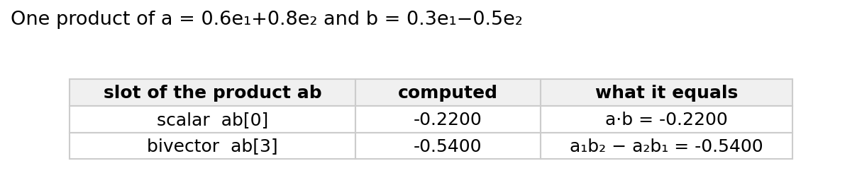
The scalar part is −0.2200, which equals 0.6·0.3 + 0.8·(−0.5). The bivector part is −0.5400, which equals 0.6·(−0.5) − 0.8·0.3. A single multiplication performed both the dot product and the signed area at once and kept them in separate components, so either can be recovered. This is the reframing in its simplest form. The geometric product is the familiar dot product together with the part that linear algebra ordinarily discards.

The following observation keeps the claim precise. The geometric product is bilinear, meaning it is linear in each argument separately. A bilinear map is determined entirely by its action on pairs of basis blades, and the product of two blades is always a single signed blade, obtained by sorting the generators, canceling repeats with the squaring rule and tracking the sign. Collecting those signs into one three-index table 𝒞, the Cayley tensor, expresses the whole product as a single contraction:

For the three-dimensional algebra Cl(3,0) there are m = 8 blades, so 𝒞 is an 8×8×8 array in which every entry is −1, 0 or +1. The array is sparse. Each pair of input blades (A, B) maps to exactly one output blade, so each (A, B) slice contains a single nonzero entry, giving 64 nonzeros out of 512, a density of 0.125. Flattened to an image, the structure is visible directly:

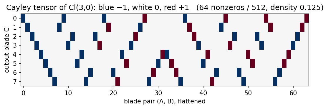
This image illustrates the position held throughout the series. No geometric-algebra library runs underneath. The call cl.geometric_product(x, y) is exactly torch.einsum('...a,cab,...b->...c', x, C, y), a single batched tensor contraction. Geometric algebra determines what the table 𝒞 must contain, and PyTorch computes the contraction using the GPU kernels, autograd and mixed precision it already provides. We claim no speed advantage and no additional expressive power for the algebra. The algebra explains why the table has the form it does, and the matrices perform the arithmetic.

This construction now settles the status of the number systems used earlier. The complex numbers and the quaternions are not merely similar to small geometric algebras. They are the small geometric algebras exactly, as algebra isomorphisms.

Take one generator that squares to −1, the signature written Cl(0,1). The map a + b·i → a + b·e₁ sends the imaginary unit i to an element that squares to −1, and it is an exact isomorphism onto a two-dimensional algebra, so Cl(0,1) ≅ ℂ. Take two generators squaring to −1, the algebra Cl(0,2), and set i = e₁, j = e₂, k = e₁e₂. Then i² = j² = −1 and k² = e₁e₂e₁e₂ = −1, while ij = e₁e₂ = k and ji = e₂e₁ = −k. These are exactly Hamilton’s relations for the quaternions, so Cl(0,2) ≅ ℍ.

A second route to the same conclusion matters for what follows. Within any geometric algebra, the even-grade blades, the scalars and bivectors and so on, are closed under multiplication, because an even blade times an even blade is again even. That even part is itself an algebra, the even subalgebra. In the Euclidean plane Cl(2,0) the even part is spanned by 1 and e₁e₂, and (e₁e₂)² = −1, so the even subalgebra of Cl(2,0) is again ℂ. By the same count, the even subalgebra of three-dimensional space Cl(3,0) is ℍ. This is not an incidental fact. It is the reason rotations in the plane are described by complex numbers and rotations in space by quaternions, because, as the next demonstration shows, the elements that perform rotations lie in the even subalgebra.

The library carries no separate complex or quaternion type, and it needs none, because the carriers used by RotatE and QuatE are these Clifford algebras. The claim can be verified by computing both products on the same random inputs and measuring the difference. The geometric product of Cl(0,1) matches complex multiplication, and Cl(0,2) matches the Hamilton product, to floating-point noise:

Both differences are about 10⁻⁷, which is single-precision round-off, so the two computations are identical. This is why the ladder from earlier in the series was not a collection of unrelated devices. ℝ, ℂ and ℍ are Cl(p,q) at three sizes, and the rotation each one provides is a single rotation construction at three sizes, which is the subject of the next demonstration.

Consider what a rotation is in this language, beginning one level below it with a reflection. To reflect a vector x in the hyperplane perpendicular to a unit vector u, the standard formula is x → x − 2(x·u)u. Substituting the one rule, ux + xu = 2(x·u), reduces that formula to a single product:

A reflection is a sandwich, in which x is placed between two copies of u. Composing two reflections gives a rotation, so a rotation is a sandwich by a product of two unit vectors. Such products are called rotors, and a rotor R acts on a multivector X by

where R̃ is the reversion of R. Reversion is one of three sign-flipping operations that recur when scores or inverses are formed, and each is a single vector of signs in the coefficient representation. Grade involution multiplies a grade-k blade by (−1)ᵏ, reversion multiplies it by (−1)^(k(k−1)/2), and Clifford conjugation composes the two. Reversion is the operation used here, because it inverts a rotor. Its name is literal, since reversion writes the generator products in reverse order, so the reversion of e₁e₂ is e₂e₁ = −e₁e₂, which is the sign change on grade-2 and grade-3 blades that the formula predicts. Which involution belongs in a given score is a modeling choice and should be stated explicitly rather than inferred from the notation.

A rotor is constructed by exponentiating a bivector, and because a bivector squares to −1 its exponential reduces exactly as e^(iθ) does:

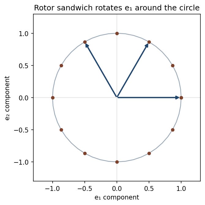
No special bivector exponential is required. Left multiplication by an element is an ordinary matrix, read directly from the Cayley tensor, and it is an algebra homomorphism, so the matrix exponential suffices. Once again the algebra names the object and linear algebra computes it. Constructing the rotor for a 60° turn in the e₁e₂ plane yields two numerical facts. It satisfies R R̃ = 1, so the sandwich is its own exact inverse, and applying it to a vector leaves the vector’s length unchanged to within 2×10⁻⁵. A rotor is therefore an isometry, a map that preserves length. Sweeping the angle, the tip of e₁ traces the unit circle:

Two further properties make rotors a suitable carrier for relations, and both are exact rather than approximate. The inverse of a rotor relation is the reversed rotor, ρ_R⁻¹ = ρ_R̃. The composition of two rotor relations is the product of the rotors, ρ_R₂ ∘ ρ_R₁ = ρ_(R₂R₁), so applying one relation and then another gives the single rotor R₂R₁. When a relation is modeled as a rotor, inversion and composition are not patterns that the geometry happens to approximate. They are algebraic identities.

The second identity explains the difference between QuatE and RotatE noted earlier in the series. In a single plane, two rotations commute, as complex numbers do. In three dimensions they do not, and the algebra records the failure directly:

The two products differ by a sign, so the rotations they generate do not commute. In the computed example the commutator of two rotors in different planes has norm 0.38 rather than zero. That sign is the reason quaternions can represent ordered composition, in which applying one relation and then another gives a result that depends on the order, while complex numbers cannot. The additional capability of QuatE over RotatE is a single minus sign in the Cayley table.

This section states the limitation of the construction precisely. A rotor sandwich fixes the origin and preserves lengths, so it is an orthogonal transformation. A translation x → x + a does neither. Consequently translation is not a rotor in the same space, and TransE is a genuinely different kind of model from RotatE rather than a special case of it. Geometric algebra unifies rotation, reflection and bilinear matching, and it draws a precise boundary at translation.

This boundary is not the end of the account, and the means of crossing it was present in the definition from the start. We permitted generators that square to +1, to −1 and to 0. A generator squaring to zero, a null direction, is the ingredient that makes a translation multiplicative once the space is embedded in a slightly larger algebra. That degenerate case is not a curiosity. It is the algebraic setting of the dual-quaternion model DualE and the degenerate-Clifford model deCal, both of which recover translation by moving to a signature with a null generator. We construct that extension in a later post, when it is needed. For now the relevant point is the boundary itself. The geometric product accounts for rotations fully and for translation not at all, and that seam organizes much of the rest of the book.

One technical point remains, since we will measure distances between embeddings. In an algebra where a vector can square to a negative number, the term norm is ambiguous, and two notions of size are in play. The coefficient norm fixes the blade basis and takes the ordinary Euclidean length of the coefficient vector, ‖X‖c² = ∑ XA². It is always positive, and it is the geometry the optimizer sees. The algebraic size ⟨X X̄⟩₀, built from the product and the conjugation, agrees with the coefficient norm in Euclidean signature but can become negative or zero once a generator squares to −1. A distance-based score must specify which it uses. Throughout the library the comparators use the coefficient norm, because it remains positive in every signature, which keeps training stable.

The core is four lines. Build the Euclidean plane, multiply two basis vectors and confirm the two facts derived above, that generators anticommute and that a Euclidean generator squares to one.

import torch
from kge.clifford import CliffordAlgebra
cl = CliffordAlgebra(2, 0)              # the Euclidean plane, m = 4 blades
a = torch.tensor([0., 1., 0., 0.])      # e1  (blade 0b01 = index 1)
b = torch.tensor([0., 0., 1., 0.])      # e2  (blade 0b10 = index 2)
print(cl.geometric_product(a, b))       # e1 e2 = [0, 0, 0, 1]   the bivector
print(cl.geometric_product(b, a))       # e2 e1 = [0, 0, 0, -1]  anticommutes
print(cl.geometric_product(a, a))       # e1 e1 = [1, 0, 0, 0]   squares to +1

The companion notebook builds the Cayley tensor from scratch, matches Cl(0,1) to ℂ and Cl(0,2) to ℍ to floating-point precision, reads the reversion signs off the blades, constructs a rotor as exp(θ e₁e₂) = cos θ + sin θ e₁e₂ and confirms that its sandwich preserves length, exhibits the two bivectors that do not commute and contrasts the coefficient norm with the algebraic norm that becomes negative under a generator squaring to −1.

▶ Run the notebook in Colab (no install)
📦 Code: github.com/asudjianto-xml/Knowledge-Graph-Geometry. Install it with pip install "kge-geometric @ git+https://github.com/asudjianto-xml/Knowledge-Graph-Geometry.git"

Geometric algebra is the design language and linear algebra is the implementation. From one rule, that the symmetric part of a product of vectors is their dot product, we obtain a multiplication that carries the dot product and an oriented area at once, recovers ℂ and ℍ exactly as its small cases and turns rotation into a sandwich whose inverse and composition are algebraic identities. None of this requires a special engine, since every product is one contraction against a fixed table of signs. The algebra explains why the carriers ℝ, ℂ and ℍ are the appropriate ones and what a rotation is, and PyTorch performs the arithmetic. Next week we put rotors to work as relation operators and introduce the rigid motion, the carrier that lets rotation and translation coexist.

Knowledge Graphs as Geometry is a free weekly series adapted from my book Knowledge Graph Embeddings as Geometric Operators.

The posts carry the intuition and the runnable code, while the book carries the full derivations. Subscribe to follow the whole argument, from a single translation to one operator that contains the entire model zoo.