Every Prediction Carries Its Own Evidence

Chapter 6 of Learning as a Geometry Discovery. An earlier chapter showed that a gradient-boosted tree ensemble is a kernel machine with a similarity learned from the labels https://agussudjianto.substack.com/p/trees-are-kernels-and-the-kernel. This chapter examines a single prediction from such a model and asks what it is made of: which historical cases supported it, how many of them effectively, whether they agreed and how far the result can be trusted. None of this is a separate explanation. It is computed from the same weights that produced the prediction.

Consider a single denied loan application for which the model reports a 50% probability of default. The natural question is why. A feature-attribution method answers with a bar chart of contributions: payment history raised the score, credit limit lowered it. That is informative, but it is not the answer a reviewer or a regulator is usually after. The answer they want has a different form. It names the most similar past applicants, states what happened to each of them and reports how much confidence the prediction deserves given how many comparable cases actually exist.

This answer requires no extra model. If the predictor is a kernel machine, and the earlier chapter established that a tree ensemble is one, then the answer is already contained in the prediction itself.

It is worth being precise about how this differs from common practice. Post-hoc explanation methods treat the model as a sealed function and fit a second model to approximate its behavior locally. SHAP constructs a local additive surrogate; LIME perturbs the inputs and observes how the output changes. Both approximate a mechanism they cannot inspect directly, and the approximation can disagree with it. A kernel machine does not work this way. Its prediction is a weighted average over training cases, and the weights themselves record how the prediction was formed. There is nothing to approximate, because the weights are the computation. This is the distinction between explaining a model after the fact and building a model whose computation is already its explanation, and the remainder of the chapter develops the second.

Recall the leaf kernel from the earlier chapter: two cases are similar to the extent that the trees of the ensemble route them to the same leaves. Placing that kernel in a Nadaraya–Watson smoother makes the prediction a weighted average of past labels:

The weights wᵢ(x) are nonnegative and sum to one, which has two consequences worth stating. First, the weights form a probability distribution over the training cases, so the prediction is a convex combination of their labels and cannot fall outside the range of the cases it averages. Second, the weight vector w(x) is itself the explanation: it records which past cases the prediction relied on and by how much. For the leaf kernel, wᵢ(x) is the share of leaf-mate evidence contributed by case i.

The remainder of the chapter is concerned with reading these weights and the quantities derived from them.

Two predictions can both be valid weighted averages while differing greatly in how much evidence supports them. One may spread its weight evenly across two hundred similar cases. Another may concentrate almost all of it on a single near-duplicate. The two are equally averages but not equally reliable. The effective sample size distinguishes them:

When the weights are uniform over n cases, N_eff = n. When all the weight falls on a single case, N_eff = 1. The quantity counts the cases that materially carry the prediction. A prediction with N_eff ≈ 160 rests on broad support. A prediction with N_eff ≈ 3 rests on very little, and should be treated with caution however confident the reported score appears.

The two extremes make the quantity concrete. Suppose that after sharpening and keeping the top 200 cases the surviving weights are nearly equal, about 1/200 each. Then Σᵢ wᵢ² ≈ 200·(1/200)² = 1/200 and N_eff ≈ 200, so the prediction is a consensus of roughly two hundred cases. Suppose instead that one case is far more similar than the rest and receives 90% of the weight. Then Σᵢ wᵢ² ≈ 0.9² = 0.81 and N_eff ≈ 1.2, so the average is essentially a single case. The reported score can be identical in both situations. N_eff is what distinguishes the consensus from the near-duplicate.

Counting the supporting cases is only part of the picture. The other part is whether they agree. The local label spread

is large when the supporting cases disagree on the outcome. A credit prediction can rest on two hundred comparable applicants and remain unreliable if those applicants divide evenly between defaults and non-defaults. N_eff measures how much evidence supports the prediction; Δ_y measures how consistent that evidence is. The two describe different failure modes. Small N_eff indicates that few comparable cases have been observed. Large Δ_y indicates that many have been observed but they disagree. The first warrants caution about extrapolation. The second warrants attention to whichever feature is dividing the neighborhood.

These quantities have a familiar counterpart. The Gaussian process posterior of the previous chapter assigns each prediction a variance that grows where training data is sparse. N_eff and Δ_y capture the same information for a smoother rather than a probabilistic model, at negligible computational cost.

The same weights can be used to audit the ensemble that produced them. Write q for the score the ensemble assigns a case and call it the teacher. One can ask whether the teacher’s score at the query is consistent with its scores on the query’s neighbors. The teacher-fidelity gap measures the discrepancy:

A small G_q means the ensemble scored the query as it scored its neighbors. A large G_q means the ensemble placed the query where its own neighborhood does not support it, which is a local signal of unreliability. The gap is not an arbitrary quantity. A short Cauchy–Schwarz argument bounds it:

The right-hand side is the spread of the teacher’s scores among the neighbors. The smoother therefore agrees with the teacher whenever the teacher is stable across similar cases, and a large gap necessarily reflects a heterogeneous neighborhood. Because the bound is exact, G_q is a defensible trust flag rather than an informal diagnostic.

A final quantity is the local calibration residual, C_cal(x) = Σᵢ wᵢ(x)·(yᵢ − qᵢ). A positive value indicates that the teacher under-predicts in this region and a negative value that it over-predicts. Together these give a simple rule for flagging a prediction as low-confidence: small N_eff, or large Δ_y, G_q or |C_cal|.

The aggregate quantities are useful, but the object a reviewer reads directly is the list of witnesses: the most heavily weighted training cases, each shown with its weight, its outcome, the teacher’s score and the kernel distance. These are the precedents the prediction rests on, and the weight is the strength of each.

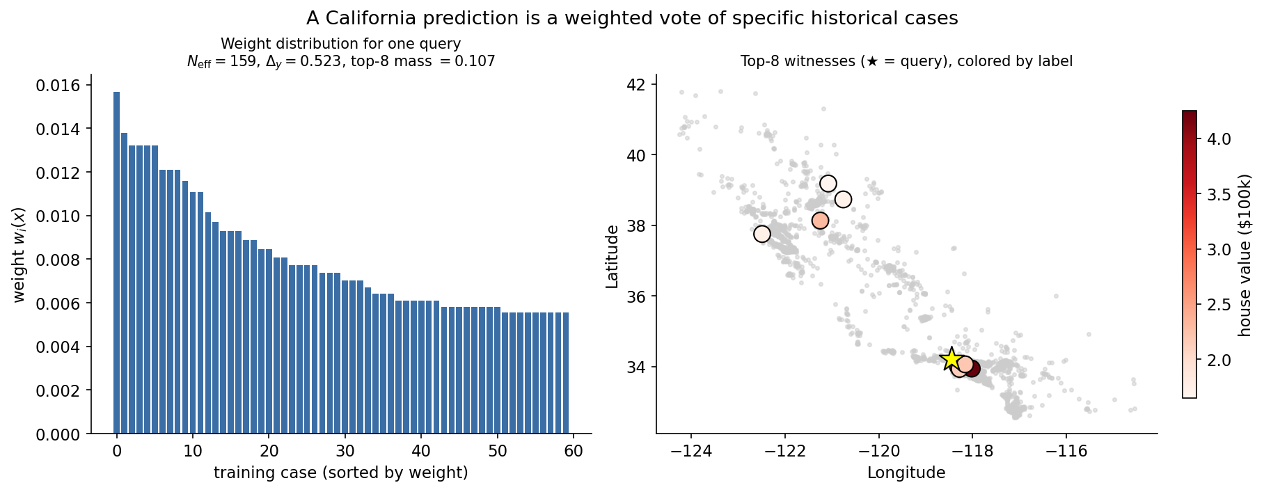
The left panel shows the sorted weights for one California prediction; N_eff is visible in how slowly the tail decays. The right panel places the eight heaviest witnesses on the map, colored by house value, with the query marked by a star. The prediction is a weighted reference to those specific nearby cases. The full ledger for the same house follows.

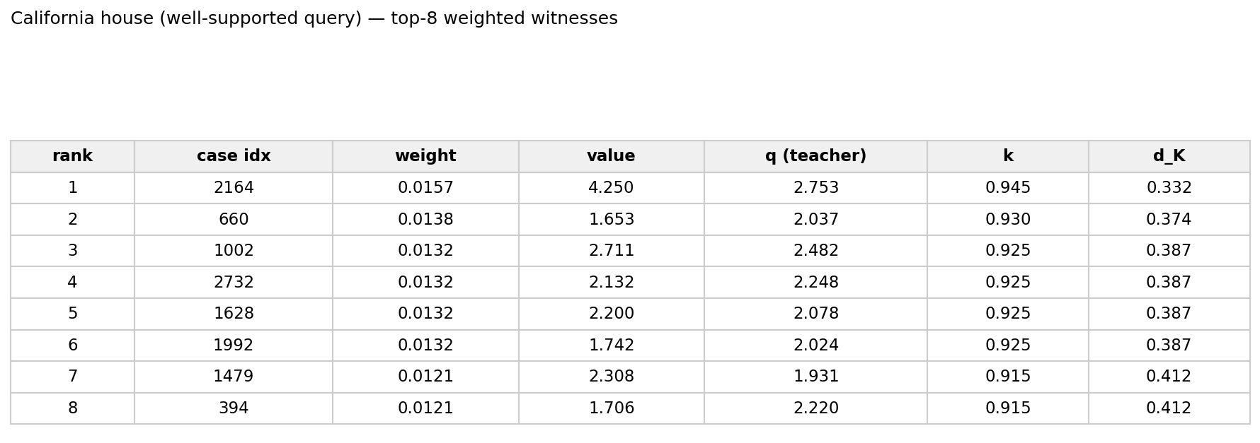
The ledger reports the local mean of about $240k, an effective sample size of 159 indicating broad support, a teacher-fidelity gap of 0.00 indicating that the ensemble agrees with the neighborhood and eight comparable blocks whose values cluster around the prediction. The case indices refer to actual training rows, so the underlying records can be retrieved. This is an explanation obtained as a byproduct of the prediction rather than from a separate model fitted afterward.

The weight formula contains a second parameter, the exponent β. At β = 1 the weights are proportional to the raw leaf similarity, which on these datasets is diffuse: the top eight witnesses hold about 5% of the total mass and N_eff sits near the truncation limit of 200. Larger β rewards the closest cases more steeply. At β = 8 the top eight hold about 11% of the mass and N_eff falls into the 150s. Validation selects β = 8 on both datasets, since a sharper vote concentrates on genuinely comparable cases without collapsing onto one.

β is the kernel-machine analogue of the temperature in an attention layer, where a low temperature concentrates attention on a few keys and a high temperature averages over many. It is selected by held-out loss rather than by preference. Its value is also visible in the ledger, since it sets how concentrated the witness list is. A preference for a tighter set of precedents and a preference for a broader consensus are, in effect, disagreements about β that the data resolves.

So far the prediction has averaged the observed labels yᵢ. The witnesses admit three natural choices for what to average:

• Empirical: average the observed labels, Σᵢ wᵢ·yᵢ. This is the most transparent choice.

• Teacher: average the ensemble’s scores, Σᵢ wᵢ·qᵢ. This has lower variance and explains the teacher.

• Blended: average a mixture zᵢ(ρ) = (1−ρ)·yᵢ + ρ·qᵢ, with ρ chosen on a validation fold.

ρ = 0 recovers the empirical head and ρ = 1 the teacher head, with held-out data selecting the value in between. The selected value differs sharply across the two datasets.

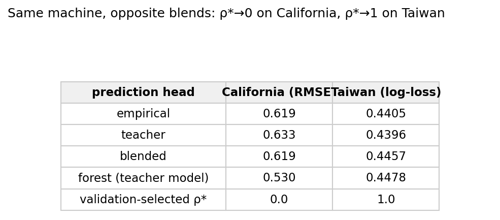
On California Housing validation selects ρ → 0. The house values vary smoothly in the supervised geometry, so averaging the observed labels is the better target and the blend defers to them. On Taiwan Credit validation selects ρ → 1. Defaults are binary outcomes with substantial noise within each leaf, so averaging the teacher’s calibrated probabilities is preferable to averaging the raw indicators and the blend defers to the teacher. The model class, the kernel and the validation rule are identical in both cases. The selected ρ* reflects the noise regime of the data.

The reversal follows from what is being averaged within a leaf. On California the labels are continuous house values and the leaf-mates carry low-noise signal, so the observed yᵢ are the most direct evidence available and the teacher’s score is a smoothed version of the same information. Averaging the raw labels is better because there is little noise to remove. On Taiwan the labels are binary, and within a neighborhood of similar applicants some default and some do not, largely at random. Averaging those indicators carries that irreducible noise into the prediction, whereas the teacher’s score is already a smoothed probability. Averaging the teacher’s probabilities is then the lower-variance estimator. In both cases the blend selects the lower-variance estimator, and which one that is depends on how noisy the labels are at the scale of a leaf.

A practical consequence is that the noise level of the labels need not be known in advance. Fitting the blended head on a validation fold and reading off ρ provides an estimate of it: a value near zero indicates that the labels are reliable at the leaf scale and a value near one indicates that they are noisy and the smoothed teacher should be preferred. ρ functions as a measurement rather than a hyperparameter to be guessed.

The Taiwan ledger for a borderline applicant, one whose blended probability is close to 0.5, illustrates this.

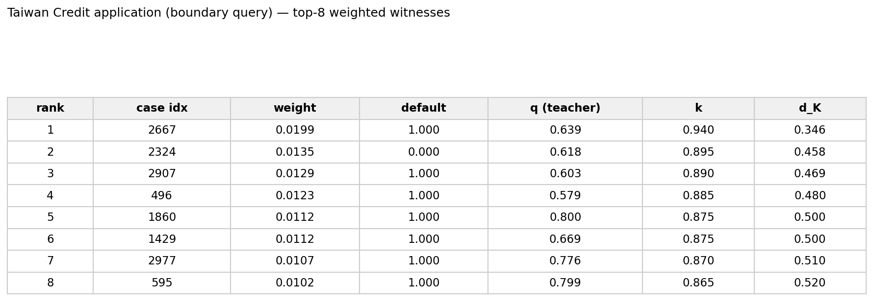
Its effective sample size is 164, indicating broad support, but its label spread is Δ_y = 0.25, meaning the witnesses are divided on whether they defaulted. The large spread identifies the case as genuinely low-margin, information the ledger makes explicit rather than concealing behind a probability of 0.50. The teacher head here reproduces the ensemble’s log-loss closely (0.4396 against 0.4478), so the accuracy is retained together with the supporting evidence.

A smoother is well calibrated where its evidence is dense and unreliable where it is sparse, and N_eff identifies which regime each query is in.

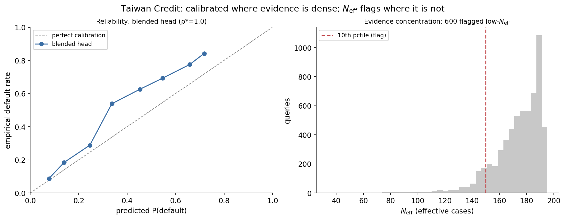
The left panel shows the reliability curve of the blended head on Taiwan Credit, plotting predicted default probability against observed default rate; it lies close to the diagonal where the bins are well populated. The right panel shows the distribution of N_eff across the test set, with the lowest decile flagged. These low-N_eff predictions are the ones a deployment should route to human review, not because the score is necessarily wrong but because the model has too few comparable cases to be confident.

The construction illustrates a position that runs through this series. In high-risk applications the explanation should be the model’s own computation and not a separate account of it. The two options are usually distinguished as intrinsic interpretability and post-hoc explanation, and the difference has practical weight. A post-hoc method reports an approximation of the model, and an approximation can be unfaithful to the decision it describes, unstable under small changes in the input and sensitive to its own configuration. When a decision must be defended to an applicant or a regulator, an explanation that can differ from the actual decision is a liability, because the institution has deployed one function and justified another.

The evidence ledger closes that gap because the object deployed is the interpretable one. The prediction is the weighted vote, and the witnesses, N_eff, Δ_y, G_q and C_cal are all quantities within that same vote, so the explanation is exact rather than approximate. The teacher-fidelity bound sharpens the point. G_q is provably small whenever the neighborhood is homogeneous, so the agreement between the reported evidence and the ensemble’s score is a guaranteed property and not an empirical hope. Post-hoc methods provide no comparable guarantee.

The standard objection to intrinsic interpretability is that it costs accuracy. The evidence here is mixed and instructive. On Taiwan Credit, a noisy binary-outcome problem of the kind common in high-risk settings, the interpretable head matches the ensemble’s log-loss (0.4396 against 0.4478). On California Housing, where the labels are cleaner, the smoother gives up accuracy relative to the ensemble (an RMSE of 0.619 against 0.530). The pattern is not accidental. Where outcomes are noisy, averaging comparable cases is close to the best any estimator can do, so little is lost by using the readable one. Where the signal is clean, a less constrained model can extract more. In the noisy regulated settings this book is chiefly concerned with, the interpretable model is not the weaker choice.

For a model-risk function the requirements are specific. A review of a denied application needs a reason for the decision, the precedents that support it and a defensible statement of confidence. The ledger supplies all three from the prediction itself. The witnesses are the precedents, identified by case. N_eff and C_cal form the confidence statement. Δ_y and G_q are named failure modes a validator can examine and challenge. This is the same principle applied earlier in the series, where a monotone functional-ANOVA model was read directly through its effect shapes and a mixture of experts repaired a weak region without leaving the interpretable family. The recurring choice is to read the model rather than to approximate it. A fuller audit artifact is developed later in the series, but the essential machinery is already present in the few lines of code below.

The entire ledger is a dozen lines of NumPy on top of the earlier chapter’s kernel. The same weights feed the prediction and every diagnostic:

W = nw_weights(K_qt, topk=200, power=beta)     # row-stochastic NW weights
pred    = W @ y_train                           # the weighted vote
neff    = 1.0 / (W**2).sum(axis=1)              # effective sample size
delta_y = W @ (y_train**2) - pred**2            # local label spread
g_q     = abs(q_query - W @ q_train)            # teacher-fidelity gap
c_cal   = W @ (y_train - q_train)               # local calibration
# top-k witnesses: sort each row of W, gather (index, weight, y, q, kernel, distance)

The companion notebook builds both ledgers, reproduces the ρ → 0 and ρ → 1 results and provides a slider for stepping through any query’s evidence while N_eff, Δ_y and G_q update.

▶ Run it in Colab (no install): open in Colab

📦 Code: github.com/asudjianto-xml/Learned-Kernel

The leaf kernel and the teacher score are introduced in Trees Are Kernels — and the Kernel Knows Where the Model Is Weak.

A kernel machine predicts by weighting historical cases, so each prediction already carries its own evidence: the cases it used, how many of them effectively, whether they agreed and whether the model’s own score is faithful to them. Interpretability here is not an added component. It is the arithmetic of the prediction read in the reverse direction. The next chapter turns to selecting the kernel and its parameters without leakage.

The Learning is a Geometry Discovery is a free weekly series adapted from my book of the same name. The posts carry the intuition and the runnable code; the book carries the full derivations.