From Chosen to Learned Kernels

Chapter 3 of The Learned Kernel. Last time, five methods collapsed into one machine whose only real input is the kernel. This time we stop choosing that kernel by hand — and confront the two things that go wrong the moment you try to learn it instead.

Every kernel tutorial begins the same way: choose a kernel, set its bandwidth. We have spent two posts arguing that this first step is the whole model in disguise — that the kernel is the geometry, and the geometry is what carries the prediction. So here is the uncomfortable question that follows. If the bandwidth decides how good your model is, why are you setting it by hand?

Let me show you just how much that one number decides, then turn it from a setting into something the data fit for themselves. The catch is that learning a geometry is not as simple as running an optimizer over it. Two hazards appear that a fixed kernel never has to face, and most people who “tune their kernel” walk straight into both. By the end of this post you will know what they are and how to disarm them.

One note on scope. The kernel we learn here is the simplest one there is — a Gaussian RBF with a length scale per feature. That is deliberate: it is the cleanest setting in which to see what learning a geometry actually means, and the two hazards below appear in their plainest form. The more flexible kernels, and the sharper geometric discovery they buy, come in later posts.

Take the Gaussian kernel and do the usual thing — pick a bandwidth ℓ — except instead of picking, sweep it across two orders of magnitude and watch the test error on the California housing data.

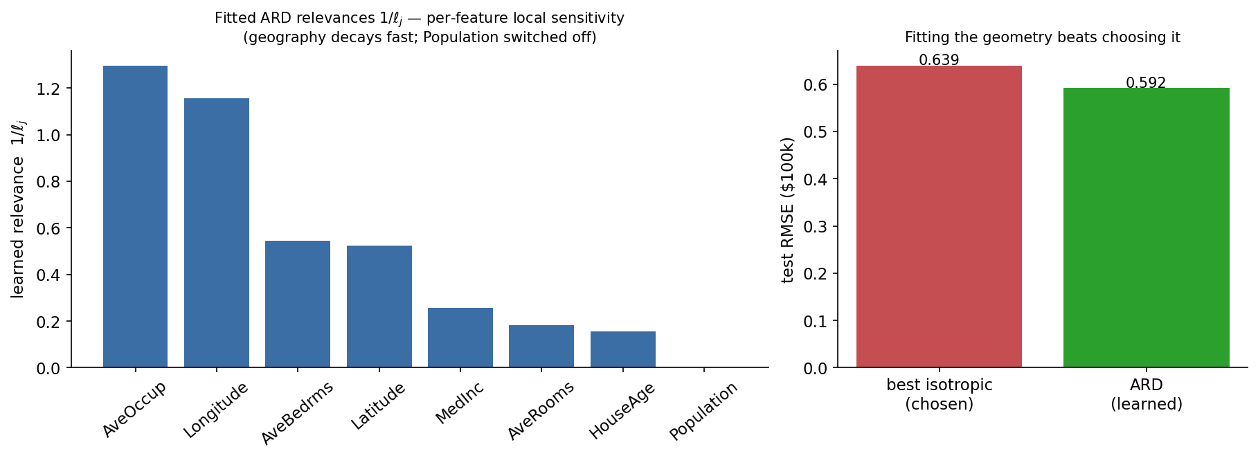
The curve is a deep U. Too narrow (ℓ = 0.1) and every test point sits alone in its own spike with no neighbors to learn from: RMSE of $118k. Around ℓ = 2 the bandwidth matches the scale of real structure and the error falls to $63k. Too wide and it smooths everything back into mush. Best beats worst by $55k in typical error — produced by nothing but the choice of a single number.

Sit with that. The bandwidth was never a tuning detail you set and forget. It was silently carrying the entire difference between a useful model and a useless one, under the polite label of “hyperparameter.” And the rule is simple: if a number moves performance that much, it is not a setting. It is a parameter. The only principled thing to do with a parameter is to learn it.

One bandwidth forces every feature to share a scale, which is almost never right. In California, geography varies on a neighborhood scale while income varies smoothly across the whole state — why force them through the same ruler? Give each feature its own length scale ℓ_j. This is the ARD kernel (automatic relevance determination):

k_θ(x, x’) = exp(−½ Σⱼ₌₁ᵈ (x_j − x’_j)² / ℓ_j²), θ = (ℓ_1, …, ℓ_d)

A small ℓ_j makes the kernel pay close attention to feature j; a large one flattens it; ℓ_j → ∞ removes the feature entirely. The metric is now anisotropic, and every ℓ_j is a number we can fit — so fit them, by minimizing error on a held-out fold.

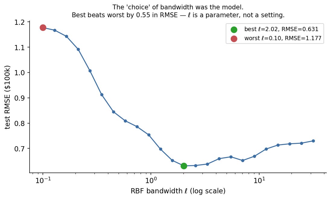
Two things to read off. On the right, the learned anisotropic geometry reaches a test RMSE of 0.592 against 0.639 for the best single isotropic bandwidth the sweep could find — fitting the geometry beats choosing it, even after the choosing was done optimally. On the left, the fitted relevances 1/ℓ_j: geography and average occupancy decay fastest, and Population is switched clean off, which is right — the raw headcount in a block says little about the value of a house in it.

One reading needs care, because this is where ARD is most often misread. The relevance 1/ℓ_j measures local sensitivity — how fast the target changes as you move along feature j — not raw importance. Median income lands low not because it does not matter but because its effect is smooth: value rises with income across the whole range, a long, gentle trend the kernel captures with a large ℓ. Geography ranks high because the spatial effect is genuinely wiggly at the neighborhood scale. So 1/ℓ_j ranks features by the roughness of their effect. It is an inspectable description of the geometry the model learned — just not a naive importance score.

ARD is the simplest learnable family, not the last. Deep kernels and the spectral mixtures of later chapters extend the same move: a kernel is a function k_θ, and learning means fitting θ. But before fitting anything, there is a trap.

Here is a fact that should make you nervous about fitting the kernel and the ridge λ together. Scale the whole kernel and the ridge by the same constant α and the kernel-ridge prediction does not change at all:

(αK)(αK + αλI)⁻¹ = (αK) α⁻¹(K + λI)⁻¹ = K(K + λI)⁻¹

The α cancels. Double the kernel and double the ridge and the prediction is identical to the last digit:

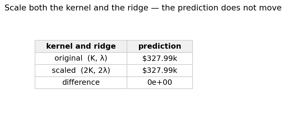
So the overall scale of the kernel and the size of the ridge are not separately identified — they trade off along a whole ridge of equivalent models. Turn an optimizer loose on both and it wanders that ridge; the λ it reports means nothing on its own.

The fix is a convention, and every kernel in this book obeys it from here on: constrain the diagonal to one, k_θ(x, x) ≡ 1. The ARD kernel already does, since exp(0) = 1. Fixing the diagonal removes the one free scale knob, so λ becomes identifiable and the held-out loss has a unique best λ instead of a flat valley. It also survives mixing: a convex combination of unit-diagonal kernels is still unit-diagonal, so when we fuse geometries in later chapters, λ stays meaningful. That is the easy hazard handled. The hard one is not about scale at all.

There are two distinct ways a learned kernel can fool you, and conflating them is the most common mistake in the whole area.

The first is overfitting the function: a flexible fit chases the noise in the labels. Everyone knows this one, and the ridge λ is its cure — turn λ up and the fit smooths out. Tuning λ on held-out data is uncontroversial.

The second is overfitting the geometry, and λ does nothing for it. A flexible kernel family can reshape the metric itself to flatter the training labels — it can decide, after the fact, that the features which happen to separate this particular sample are the important ones. The sharpest case is the boosted tree of the next post: it grows its leaves to fit the residuals, so the kernel it induces nearly interpolates the training labels by construction. Score that kernel on the training set and it looks magnificent at any λ — because turning up λ smooths the function while leaving the geometry, which already memorized the labels, untouched. The leakage is baked into the kernel matrix itself, fit from the very labels you are about to grade it on. No amount of ridge fixes a ruler that was bent to the answer.

The conclusion is forced: you cannot choose the geometry with any criterion that lets the kernel see the labels it is scored against. You have to fit it on one split and judge it on another — which is exactly the held-out fold we used to fit the ARD scales above. That is not a nicety. It is the only thing standing between learning a geometry and memorizing one, and it is why the relevances in that chart describe the data rather than the fit. (The full leakage-free theory — what to hold out and the guarantee it buys — is a later chapter.)

From here the book is a sequence of engines for fitting the geometry, each one forced by this post. Boosting fits a leaf geometry straight from the labels — the forest was a learned kernel all along (next time). The marginal likelihood gives a kernel a score to maximize. And amortized inference learns a network that emits a kernel from a handful of examples in a single forward pass, with no per-dataset training at all. Different engines, one target: discover the geometry instead of declaring it. Each will have to answer the two questions this post raised — is the fit identifiable, and is it scored without leakage.

The whole chapter is a sweep and a fit:

def ard_gram(A, B, ell):              # per-feature length scales; diagonal = 1
    Aw, Bw = A / ell, B / ell
    d2 = ((Aw**2).sum(1)[:,None] + (Bw**2).sum(1)[None,:] - 2*Aw@Bw.T).clip(0)
    return np.exp(-0.5 * d2)
# fit log(ell_j) by minimizing error on a HELD-OUT fold — never the fold that built K

The companion notebook runs the bandwidth sweep, fits the ARD scales on a held-out fold, verifies the scale degeneracy is exact, and gives you a slider to pick a bandwidth by hand and watch it lose to the learned geometry.

▶ Run it in Colab (no install): open in Colab

📦 Code: github.com/asudjianto-xml/Learned-Kernel

The previous installment, The Kernel as the Normal Form, is where “the kernel is the only choice” comes from.

The geometry is the output, not the input. Once you accept that, the bandwidth stops being a knob you turn and becomes a parameter you fit — under two disciplines, identifiability and leakage-free scoring, that a chosen kernel never needed. Next week: the gradient-boosted tree, which has been learning a kernel from your labels this whole time without telling you.

The Learned Kernel is a free weekly series adapted from my book of the same name. The posts carry the intuition and the runnable code; the book carries the full derivations.