A Relation in Knowledge Graph Is a Matching Matrix

This is the third post in Knowledge Graphs as Geometry, a weekly series that builds one idea, chapter by chapter: a knowledge graph stores facts as relations, every relation is an operation in space, and predicting a missing fact is geometry. Every post runs on a real (if tiny) graph, and the full, executed code is one click away at the end.

Back to the family. Ann and Bob are married and parent two children, Carol and Dave; Carol married Eve, and they have Frank. Last week we scored a fact the way TransE does — by distance https://agussudjianto.substack.com/p/transe-translation-as-a-decoder. Build a prediction 𝐡 + 𝐫, and ask how far the tail lands from it. That worked, but it ran into a wall: a translation cannot represent a symmetric relation without sending it to zero. spouse broke it.

This week we follow the other great family of models, and they start from a completely different instinct. They do not measure distance at all. They measure agreement. Instead of asking “how far is the translated head from the tail,” a bilinear model asks “how well do the head, the relation and the tail line up.” Same task — answer (Ann, parentOf, ?) with Carol and Dave — but a different geometry underneath. And it is this family, not TransE, that finally gives a clean answer to the symmetric-relation question.

The catch is that the most natural version of it trades one blind spot for another. TransE could not do symmetry; the simplest matching model will turn out to do only symmetry, which is just as crippling for a graph full of directed facts. The repair is one of the most important moves in the whole book, and it is not the obvious one. We do not give the model a bigger, more expensive operator. We change the number system the coordinates live in — and the same cheap operator that failed suddenly works. That is the first appearance of the carrier, the first of the three choices the series turns on, and it is worth watching closely because the same move recurs again and again as we climb through the zoo.

A word on why this is worth four demonstrations rather than one. The bilinear family is not a single model but a lineage — RESCAL, DistMult, ComplEx, TuckER — and each member is usually taught as its own method with its own paper and its own scoring rule. The thesis of this series is that they are not separate at all. They are one scoring template seen at four settings of a single knob, and the knob has a name we can point at in code. Watching the lineage from the top, with the knob in view, turns four formulas into one idea with four dials. That is the payoff for going slowly here.

Give every entity a vector, just as before. But now make each relation a matrix Mᵣ, and score a triple by sandwiching that matrix between the head and the tail:

Read Mᵣ as a compatibility test. The entry (Mᵣ)ᵢⱼ says how much feature i of the head should agree with feature j of the tail for the relation to hold. Multiply head feature i by tail feature j, weight it by (Mᵣ)ᵢⱼ, and add it all up. A high score means the head and tail align in exactly the way the relation demands. This is RESCAL, and with no constraints on Mᵣ it is the most expressive model in the family — it can encode any pairwise interaction between head and tail features.

That power has a price, and the price sets up everything that follows. A full matrix costs d² parameters per relation. On a real graph with thousands of relations and d in the hundreds, the relation tensor dwarfs the entity table and the model memorizes instead of generalizing. It has so many free knobs that it can fit the training facts perfectly and still rank random nonsense at test time. So the whole chapter becomes a search for the right constraint on Mᵣ: enough structure to generalize, enough freedom to keep the relations the data actually contains. Every famous model in this family is one answer to that question — a different shape carved out of the full matrix. DistMult keeps only the diagonal. ComplEx keeps a particular pattern of 2×2 blocks. TuckER routes all of them through a single shared core. The art is not in adding power; it is in choosing what to throw away.

The most aggressive constraint is to throw away everything off the diagonal. Let Mᵣ = diag(𝐫), a matrix with the relation vector on its diagonal and zeros elsewhere. The relation is a vector again, but now it scales each coordinate instead of translating it, and the sandwich collapses into a clean three-way product:

This is DistMult, and the last form is the one to keep. The relation acts on the head by the channelwise product 𝐡 ⊙ 𝐫 — multiply coordinate by coordinate — and then we take the plain inner product against the tail. We met both pieces in the library already: the product is the operation on the head, the inner product is the matching comparator. DistMult is exactly their composition. It is cheap, it generalizes well, and for a while it was the workhorse of the field.

But the diagonal buys a hard limitation, and you can see it without training anything. Look at a single term: hᵢ rᵢ tᵢ. Swap the head and the tail — swap hᵢ and tᵢ — and the term is unchanged, because multiplication does not care about order. So the whole sum is unchanged. DistMult gives a fact and its reverse the identical score, for every relation, no matter what it learns:

There is a one-line matrix version of the same fact, for the reader who likes it crisp. A diagonal matrix is symmetric — it equals its own transpose — and for any symmetric Mᵣ the sandwich satisfies 𝐡ᵀ Mᵣ 𝐭 = 𝐭ᵀ Mᵣ 𝐡. Symmetry of the matrix forces symmetry of the score. The diagonal was a convenient way to save parameters, and it quietly smuggled in a constraint nobody asked for.

In the family graph parentOf is the opposite of symmetric. Ann is a parent of Carol; Carol is emphatically not a parent of Ann. Yet DistMult is forced to score (Ann, parentOf, Carol) and (Carol, parentOf, Ann) exactly alike. It literally cannot tell a relation from its reverse — not because it failed to learn the difference, but because the difference is unrepresentable in its geometry. Train it and read the two scores off:

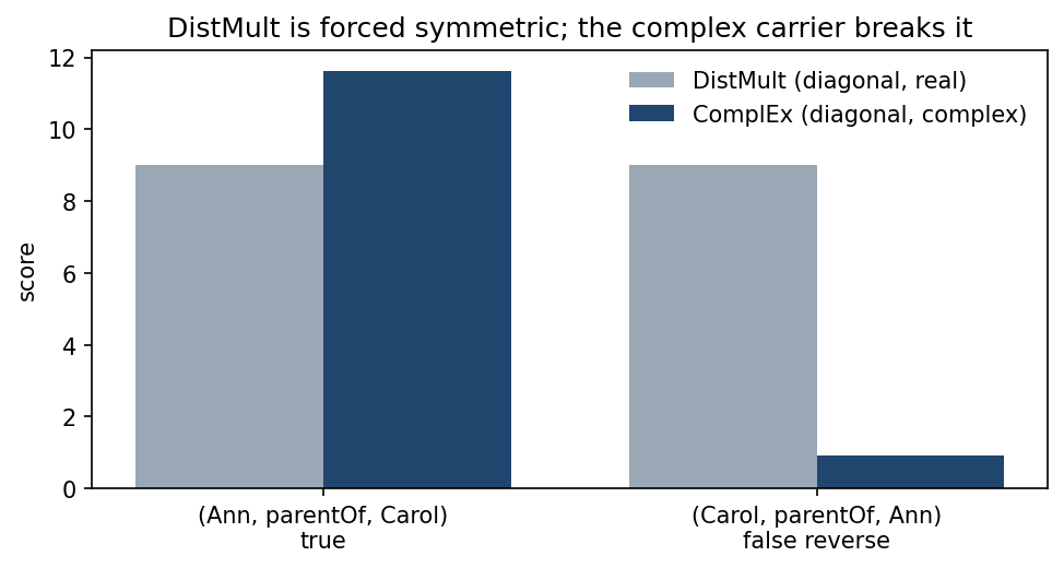
The two gray bars are equal to four decimals — both 9.002. That is not a training artifact you could fix with more epochs; it is the diagonal made visible. Where TransE was forced to send symmetric relations to zero, DistMult is forced to make every relation symmetric. Each model’s elegance is exactly its blind spot. DistMult handles spouse and siblingOf, which really are symmetric, and fails on every directed relation — which is most of the relations you actually care about.

The blue bars are the fix, and they are the rest of this post.

Here is the move. The instinct, when a model is too weak, is to give it a bigger matrix — climb back toward RESCAL and pay the d² price. The bilinear family does something far cheaper and far more interesting. It keeps the diagonal operator — still one multiplier per channel — but lets the coordinates be complex instead of real. Each entity and relation now lives in ℂ, and the score takes the real part of a three-way product with the tail conjugated:

This is ComplEx. The only change from DistMult is the bar over tᵢ — the conjugate on the tail — and that conjugate is the entire story. Conjugation is not symmetric when you swap the head and the tail, so the forced symmetry that trapped DistMult is simply gone. Train ComplEx on the same family graph and score parentOf both ways, and you get the two blue bars in the figure above: the true direction scores 11.63, the false reverse scores 0.91. The model now prefers the truth by more than ten points, with the same diagonal operator that could not separate them at all in real coordinates.

That deserves to land. We did not make the operator stronger. We changed the space it operates in, and a structural limitation dissolved. This is the first concrete payoff of separating the operator from the carrier — of treating “what the relation does” and “what kind of number a coordinate is” as two independent knobs. Hold the operator fixed at a diagonal, swap ℝ for ℂ, and a model that could not represent direction suddenly can.

We can even watch where the model files the asymmetry. Write each relation channel as rᵢ = aᵢ + i bᵢ, a real part and an imaginary part. Expand the ComplEx score and it splits cleanly: the real parts aᵢ carry a piece that is symmetric in the head and tail, and the imaginary parts bᵢ carry a piece that flips sign when you swap them. A purely real relation is symmetric; a purely imaginary relation is antisymmetric. So a well-trained ComplEx should keep its symmetric relations mostly on the real axis and spend imaginary weight only where it needs to encode a direction. We can read that balance straight off the learned vectors:

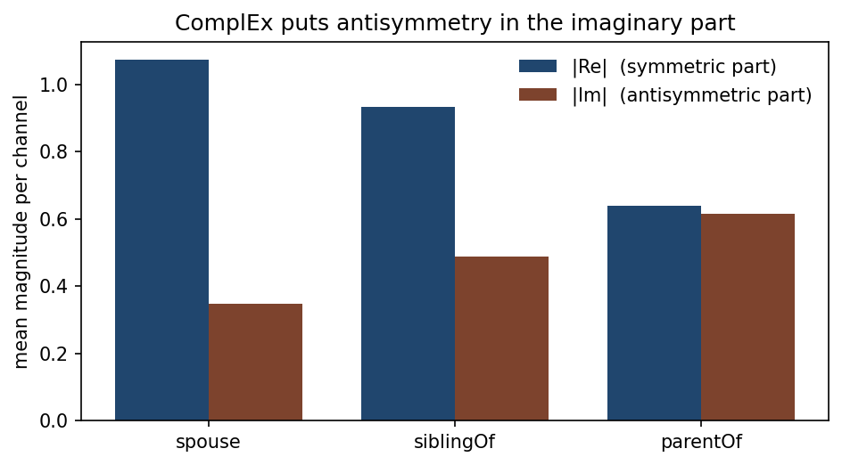
The two genuinely symmetric relations, spouse and siblingOf, are real-dominated — short brown bars. parentOf carries by far the largest imaginary share: its real and imaginary magnitudes are nearly equal, an imaginary share of 0.49 against 0.24 for spouse. The model put the asymmetry exactly where the math says it has to go. Nobody told it to. It learned that parentOf needs to tell a direction from its reverse, and the only place to store that is the imaginary part.

There is a second way to see what ComplEx bought, and it connects straight back to RESCAL. Each complex multiplication hᵢ rᵢ is, in real coordinates, a 2×2 matrix acting on the pair (real, imaginary):

\begin{bmatrix} a & -b \\ b & a \end{bmatrix}

That block is symmetric only when b = 0 — only when the channel is real. The moment b is nonzero the block has an antisymmetric part, and antisymmetry in the matrix is exactly what the score needs to tell a fact from its reverse. So ComplEx is nothing but a bilinear model whose relation matrix is block-diagonal, with each 2×2 block allowed to rotate as well as scale. Compare that to RESCAL, which allowed any d×d matrix and paid for it. ComplEx allows only this one restricted family of blocks. It buys exactly the expressiveness it needs over DistMult, and not a feature more. That is the whole trick, and it is why ComplEx generalizes where RESCAL overfits: it is the cheapest possible escape from forced symmetry, a tiny crack of freedom opened in precisely the right place.

Step back and the two posts together have set up a clean dichotomy. TransE scores by distance: build 𝐡 + 𝐫 and measure how far the tail falls from it. The bilinear family scores by matching: transform the head — 𝐡 ⊙ 𝐫 in the diagonal case — and take its inner product with the tail. Both apply a relation-conditioned operation to the head. They differ only in how they compare the result to the tail: a norm or an inner product. That comparison is the third of the three choices, the comparator, and keeping it as its own object is what will let us turn ComplEx into RotatE next week without touching the operator at all.

The difference is not cosmetic; it leaves a measurable fingerprint. The family graph showed us the mechanism, one triple at a time. A real benchmark shows us the signature across thousands of triples. Move to UMLS — a medical knowledge graph of 135 entities, 46 relations and about 5,000 facts, small enough to train in seconds on a laptop but rich enough to mix symmetric, inverse and composition patterns. Train DistMult and ComplEx and read the filtered Hits profile — the fraction of test queries whose true answer lands in the top 1, top 3, top 10:

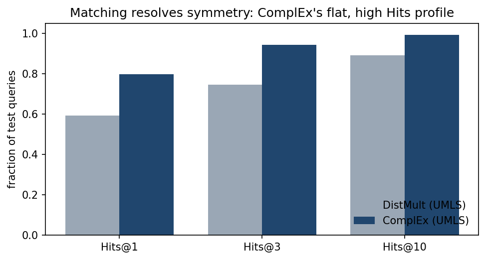
ComplEx is high and flat: 0.80 at Hits@1, 0.94 at Hits@3, 0.99 at Hits@10. If the answer is anywhere in the top three it is almost always first. That is the matching signature — a model that resolves symmetry correctly commits to a single best tail instead of leaving a cluster of plausible candidates near the top. DistMult lags everywhere (0.59, 0.75, 0.89), because every directed relation in UMLS is fighting its forced symmetry. The gap between matching and distance is even sharper on the harder WN18RR benchmark, a slice of WordNet with about 41,000 entities and only 11 relations, most of them symmetric or near-symmetric. There our ComplEx reaches a filtered MRR of 0.366 against TransE’s 0.213 — and the two profiles are mirror images. TransE is steep: it lands answers near the top (Hits@3 ≈ 0.39, Hits@10 ≈ 0.50) but almost never at it (Hits@1 ≈ 0.01), the signature of a rigid displacement that gets into the right neighborhood but cannot resolve among many-valued and symmetric relations. ComplEx is the opposite — flat and high, its Hits@1, Hits@3 and Hits@10 (0.358, 0.368, 0.382) sitting close together, because when the answer ranks at all it usually ranks first and the curve barely climbs past Hits@1. The headline MRR is that same story told once; the profile tells it relation by relation.

The shape of that profile matters more than the single MRR if you ever plan to act on a prediction. Picture the knowledge graph as the memory an AI agent reads from and writes to. When it asks (patient, hasDiagnosis, ?), a steep profile means the right answer is somewhere in a short list but you cannot trust the top of that list — you have to surface several candidates and let something downstream choose. A flat, high profile means the model’s first guess is usually the answer, so the agent can act on it directly. That is the practical difference between distance and matching here: not which one is “better” in the abstract, but which failure mode you are buying.

And notice which choice controls it. The operation on the head is the same diagonal multiply in both the steep model and the flat one — what differs is only how we compare the transformed head to the tail. A norm gives you the steep, neighborhood-finding profile; an inner product gives you the flat, commit-to-one profile. That comparison is governed entirely by the comparator, and the operation on the head is, in both ComplEx and the rotational model we meet next week, identical. So if you care about the shape of the answer list — and an agent reading from this memory does — the comparator is the dial you reach for, not the operator. This is the first time in the series that one of the three choices shows up as a directly measurable property of the predictions rather than a structural fact about expressiveness, and it will not be the last.

We have met three models — DistMult, RESCAL, ComplEx — and it would be easy to file them as three separate methods. They are not. DistMult and RESCAL are two settings of a single knob, and a third model, TuckER, makes the knob explicit. TuckER writes the entire scoring tensor through a small learned core W and shared entity and relation factors:

The core W is the same for every triple; it learns how head, relation and tail dimensions interact in general, and the embeddings specialize that pattern per entity and per relation. Now choose the core. Make W the identity superdiagonal — Wᵢⱼₖ = 1 only when i = j = k — and the triple sum collapses to Σ hᵢ rᵢ tᵢ, which is DistMult. Let W couple the relation mode to a full head-tail block and you get back RESCAL’s matrix. So the three models are a chain of increasingly free cores:

A model’s expressiveness is just how much of the core it is allowed to learn, and the parameter cost lines up exactly with that freedom:

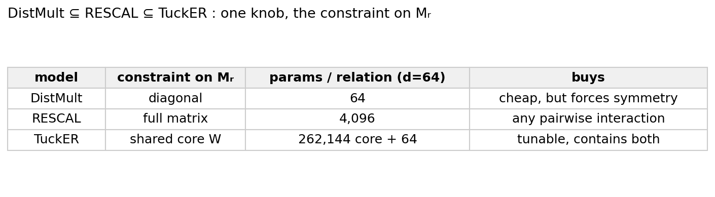
Read the table top to bottom and you can see the bias-variance ladder directly. DistMult spends 64 numbers per relation and generalizes from very little, at the cost of forced symmetry. RESCAL spends 4,096 and can represent any pairwise interaction, at the cost of overfitting when relations are many. TuckER puts the freedom in a shared core every relation reuses, so it tunes between the two. This is the first hint of the book’s central claim — that the whole zoo is one object seen at different settings. The chapter on the unified operator makes it exact: it copies a trained DistMult into a single general engine, Fᵣ(x) = Uᵣ Σᵣ Vᵣᵀ x + cᵣ, sets it to its stretch-only matching configuration, and recovers the DistMult scores bit for bit — not approximately, identically. DistMult is one row of a much larger table. We are only on the third row now.

The whole forced-symmetry phenomenon, and its repair, is a dozen lines: train both models, score a directed fact forward and backward.

from kge.data import TripleFactory
from kge.models import DistMult, ComplEx
from kge.train import Trainer, TrainConfig
import torch
triples = [("Ann","parentOf","Carol"), ("Bob","parentOf","Carol"),
           ("Ann","parentOf","Dave"),  ("Carol","parentOf","Frank"),
           ("Ann","spouse","Bob"),     ("Bob","spouse","Ann")]
g = TripleFactory(train=triples, valid=[], test=[], name="family")
def fwd_rev(Model):
    torch.manual_seed(0)
    m = Model(g.n_entities, g.n_relations, dim=16)
    Trainer(m, g, TrainConfig(mode="1vsall", epochs=300, lr=0.1), device="cpu").fit()
    s = lambda h,t: m.score_triples(torch.tensor([g.ent2id[h]]),
                                    torch.tensor([g.rel2id["parentOf"]]),
                                    torch.tensor([g.ent2id[t]])).item()
    return s("Ann","Carol"), s("Carol","Ann")   # true, false-reverse
print("DistMult:", fwd_rev(DistMult))   # equal - forced symmetric
print("ComplEx :", fwd_rev(ComplEx))    # true >> reverse

The companion notebook trains both models on the family graph, reads the real/imaginary balance off the learned ComplEx vectors, reproduces the UMLS Hits profile, and copies a trained DistMult into the unified engine to show the recovery is exact.

▶ Run the notebook in Colab : https://colab.research.google.com/github/asudjianto-xml/Knowledge-Graph-Geometry/blob/main/notebooks/ch03_bilinear_and_tensor.ipynb
📦 Code: github.com/asudjianto-xml/Knowledge-Graph-Geometry — pip install "kge-geometric @ git+https://github.com/asudjianto-xml/Knowledge-Graph-Geometry.git"

The bilinear family scores a fact by alignment, 𝐡ᵀ Mᵣ 𝐭, and is organized entirely by the constraint on Mᵣ — a full matrix is RESCAL, a diagonal is DistMult, a learned core is TuckER, and they nest. The diagonal forces every relation symmetric, and the fix is not a bigger matrix but a different number system: move the coordinates from ℝ to ℂ, conjugate the tail, and the limitation dissolves. That is the first win from changing the carrier rather than the operator. Next week: keep the complex carrier and the diagonal operator untouched, swap matching for distance, and watch ComplEx become RotatE.

Knowledge Graphs as Geometry is a free weekly series adapted from my book Knowledge Graph Embeddings as Geometric Operators. The posts carry the intuition and the runnable code; the book carries the full derivations. Subscribe to follow the whole argument — from a single translation to one operator that contains the entire model zoo.