3.1 Language Modeling: N-gram models, RNNs, LSTMs, GRUs
3.1.1 Foundations of statistical language modeling
3.1.2 Architectures of RNNs, LSTMs, GRUs
3.3.3 Training and optimization of language models
3.2 Transformers and Attention Mechanisms
3.2.1 Multi-headed self-attention
3.2.2 Transformer encoder-decoder architecture
Written in Collaboration - Special thanks to Manan Thakkar for his valuable contributions to structure this chapter, shaping it into an informative and accessible resource for understanding Advanced Language Modeling and Transformers.
In this chapter, we focuses on language modeling, which aims to predict likely next words given previous text. We first cover the foundations of statistical n-gram language models. Then, key neural network architectures for language modeling are presented, including recurrent neural networks, long short-term memory networks, and gated recurrent units. Special attention is given to transformers, state-of-the-art models that employ multi-headed self-attention to capture long-range dependencies in text. Pre-training strategies for transformers like BERT are also discussed.
By the end of this chapter, you will have strong conceptual and mathematical foundations regarding language modeling, enabling you to develop predictive NLP systems. The techniques presented form the basis for contemporary NLP with deep neural networks.
Language Modeling Foundations: Statistical n-gram models and neural network architectures like RNNs, LSTMs, and GRUs
Transformers and Attention: Multi-headed self-attention mechanisms, encoder-decoder architectures, and transformer pre-training strategies
Comparative Analysis: Contrasting different techniques for text representation and language modeling in NLP
Resources: Overview of key datasets, libraries, and learning materials on text representation and language modeling
Language modeling is a fundamental task in NLP that aims to predict the probability of a sequence of words. It plays a crucial role in various applications, such as speech recognition, machine translation, text generation, and sentiment analysis. Over the years, several techniques have been developed to tackle the challenge of language modeling, ranging from traditional statistical approaches to more advanced deep learning methods. In this section, we will explore the evolution of language modeling techniques, starting with the classic N-gram models and then delving into the powerful neural network architectures, including Recurrent Neural Networks (RNNs), Long Short-Term Memory (LSTM) networks, and Gated Recurrent Units (GRUs). We will discuss the strengths and limitations of each approach and understand how they have contributed to the advancement of NLP.
N-gram models are a classic statistical approach to language modeling that have been widely used in various NLP tasks. They are based on the assumption that the probability of a word depends only on the previous N-1 words, where N is a fixed number. In this section, we will explore the concept of N-gram models, their algorithmic implementation, and their advantages and limitations.
An N-gram is a contiguous sequence of N words from a given text or speech corpus. The key idea behind N-gram models is to estimate the probability of a word based on the context of the preceding N-1 words. The value of N determines the size of the context window and the order of the N-gram model. For example:
Unigram (N=1): Considers each word independently, without any context.
Bigram (N=2): Considers the probability of a word given the previous word.
Trigram (N=3): Considers the probability of a word given the previous two words.
The probability of a sequence of words is calculated as the product of the individual N-gram probabilities. For example, in a bigram model, the probability of a sentence "The cat sat on the mat" would be calculated as:
P("The cat sat on the mat") =P("The") × P("cat" | "The") × P("sat" | "cat") × P("on" | "sat") × P("the" | "on") × P("mat" | "the")
Algorithmic Implementation
The process of building an N-gram model involves the following steps:
Tokenization: Split the text corpus into individual words or tokens.
N-gram Generation: Create N-gram sequences by sliding a window of size N over the tokenized text.
Frequency Counting: Count the frequency of each N-gram in the corpus.
Probability Estimation: Calculate the probability of each N-gram by dividing its frequency by the frequency of the preceding (N-1)-gram.
Example: Predicting the Next Word using N-gram Model
Generated Corpus:
<S> NLP is fascinating </S>
<S> ML is a subset of AI </S>
<S> NLP and ML are important </S>
Question: Given the bigram "<S> NLP", predict the most probable next word using the bigram model.
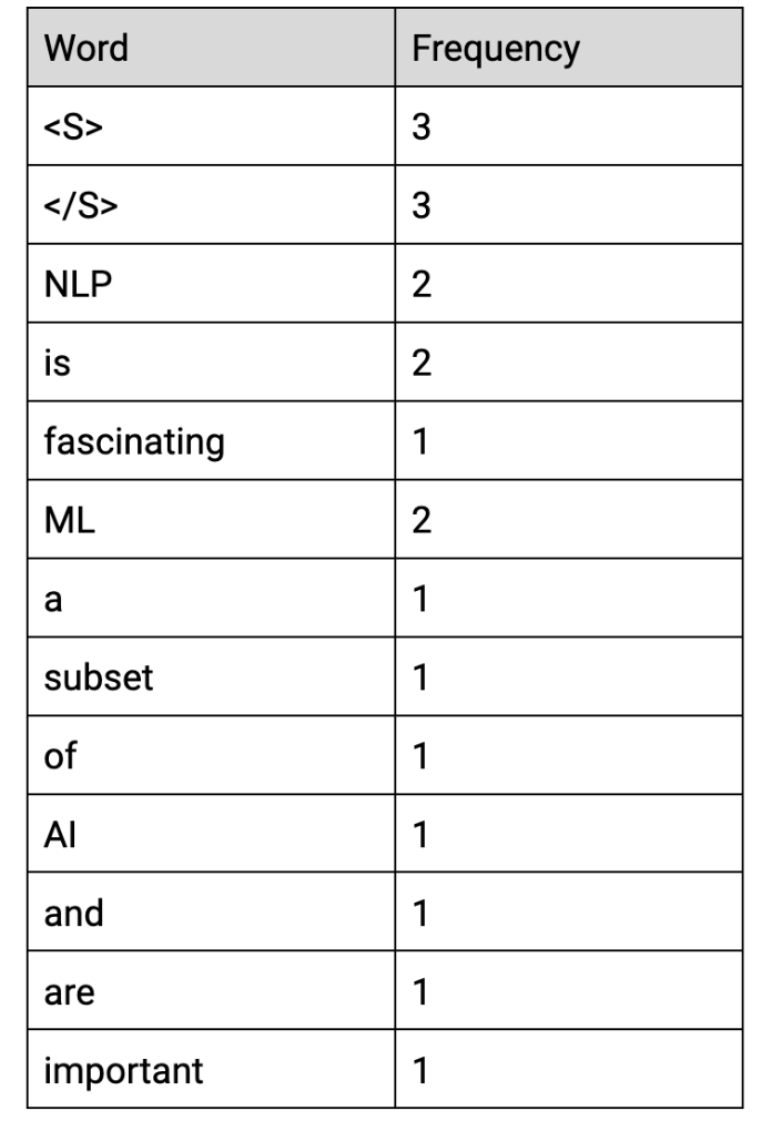
Step 1: Generate the frequency table for the corpus.
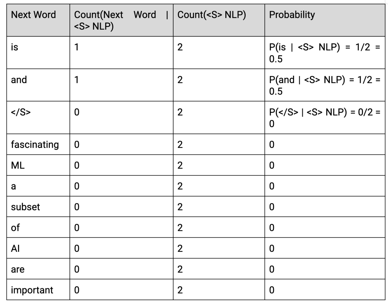
Step 2: Generate the probability table for the next word given the bigram "<S> NLP".
Step 3: Identify the most probable next word.
Based on the probability table, the most probable next words after "<S> NLP" are "is" and "and", both with a probability of 0.5.
Therefore, the most probable next words after "<S> NLP" are "is" and "and".
Code:
from collections import defaultdict
import re
def train_bigram_model(text):
# Tokenize the text
words = re.findall(r'\b\w+\b', text.lower())
# Create bigrams
bigrams = [(words[i], words[i+1]) for i in range(len(words)-1)]
# Count bigram frequencies
bigram_counts = defaultdict(int)
for bigram in bigrams:
bigram_counts[bigram] += 1
# Count word frequencies
word_counts = defaultdict(int)
for word in words:
word_counts[word] += 1
# Calculate bigram probabilities
bigram_probs = {}
for bigram, count in bigram_counts.items():
word1, word2 = bigram
bigram_probs[bigram] = count / word_counts[word1]
return bigram_probs
# Example usage
text = "The cat sat on the mat. The dog chased the cat."
bigram_model = train_bigram_model(text)
# Print bigram probabilities
for bigram, prob in bigram_model.items():
print(f"{bigram}: {prob}")
Feedforward and convolutional neural networks (CNNs) have been successful in various tasks, but they have limitations when it comes to processing sequential data. In CNNs, the input size is fixed, and each input is treated independently of the others. For example, when feeding images to a CNN for classification, the computations and decisions for two successive images are completely independent of each other.
However, many real-world problems involve sequential data, where the inputs are not of fixed size, and successive inputs may be dependent on each other. Some examples of sequence learning problems include:
Auto-completion: Given the first character 'd', predicting the next character 'e' and so on.
Part-of-speech tagging: Predicting the part of speech tag (noun, adverb, adjective, verb) of each word in a sentence.
Sentiment analysis: Predicting the polarity of a movie review based on the entire sequence of words.
In these scenarios, the current output may depend on the current input as well as the previous inputs, and the size of the input is not fixed. Traditional neural networks struggle to handle such tasks effectively.
The Need for RNNs
To address the limitations of feedforward and CNNs in handling sequential data, RNNs were introduced. RNNs are designed to handle tasks involving sequences by maintaining an internal state that allows them to capture and exploit dependencies between inputs.
RNNs have three main targets:
Account for dependence between inputs
Account for variable number of inputs
Make sure that the function executed at each time step is the same
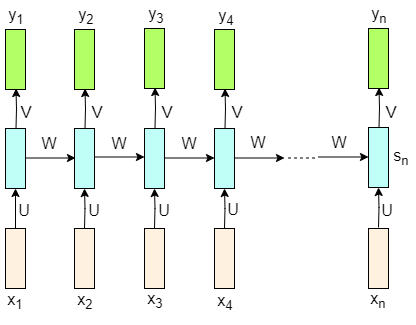
Figure – Basic RNN architecture
Recurrent Connections in RNNs
The key component of an RNN is the recurrent connection, which allows the network to maintain a hidden state that captures information from previous time steps. At each time step, the RNN takes an input and the previous hidden state, and produces an output and an updated hidden state.
The computation in an RNN can be summarized using the following equations:
where:
si is the hidden state at time step i
xi is the input at time step i
U, W, and V are weight matrices
b and c are bias vectors
is an activation function (e.g., sigmoid or tanh)
O is the output function (e.g., softmax for classification)
The recurrent connection (Wsi-1) allows the hidden state to capture information from previous time steps, enabling the RNN to handle dependencies between inputs. This recurrent connection is crucial for modeling sequential data effectively.
Training RNNs with Backpropagation Through Time (BPTT)
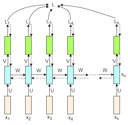
Figure – RNN with backpropagation
Training an RNN involves using the backpropagation through time (BPTT) algorithm, which unrolls the network over the sequence and applies the standard backpropagation algorithm to compute the gradients.
The total loss in an RNN is the sum of the losses over all time steps. For each time step t, the loss is computed based on the predicted output yt and the actual target c:
To update the parameters of the RNN (U, V, W), the gradients of the loss with respect to these parameters are computed using the chain rule of differentiation. The gradients are then used to update the parameters using gradient descent or its variants.
Vanishing and Exploding Gradients Problem
One of the challenges in training RNNs is the vanishing and exploding gradients problem. As the backpropagation algorithm advances backward from the output layer towards the input layer, the gradients can become very small (vanishing) or very large (exploding).
Vanishing gradients occur when the gradients approach zero, leaving the weights of the initial or lower layers nearly unchanged. This prevents the network from learning long-term dependencies effectively.
Exploding gradients occur when the gradients keep getting larger, causing very large weight updates and making the gradient descent diverge.
To mitigate these issues, techniques such as gradient clipping, using activation functions like ReLU, and more advanced architectures like LSTM or GRU can be employed.
Despite these challenges, RNNs have been widely used and have achieved significant success in various sequence modeling tasks, including language modeling, speech recognition, and machine translation. They have paved the way for more advanced architectures that further enhance the ability to capture and utilize long-term dependencies in sequential data.
RNNs have shown great success in handling sequential data, but they suffer from the problem of vanishing or exploding gradients when dealing with long-term dependencies. This limitation hinders the ability of RNNs to capture and utilize information from distant time steps effectively. To address this issue, LSTM networks were introduced.
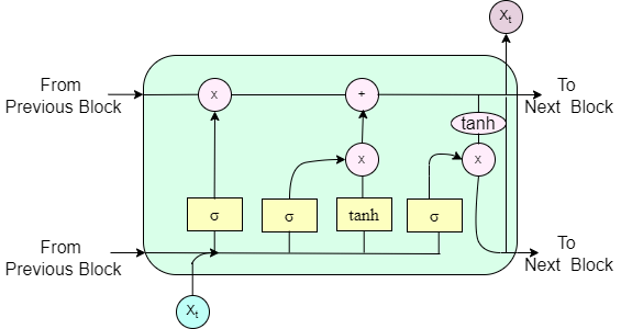
LSTM is a type of recurrent neural network architecture specifically designed to handle long-term dependencies in sequential data. It introduces a memory cell and three types of gates (forget gate, input gate, and output gate) that regulate the flow of information within the network. These components enable LSTM to selectively remember or forget information over long sequences, making it capable of capturing long-term dependencies.
Architectural Components
Figure – LSTM architecture
The LSTM architecture consists of the following key components:
Memory Cell (C):
The memory cell is the core component of LSTM that stores the long-term memory of the network.
It is responsible for maintaining the state information over time.
The memory cell is controlled by the forget gate, input gate, and output gate, which regulate the flow of information into and out of the cell.
The state of the memory cell is updated at each time step based on the outputs of the gates.
The memory cell update equation is given by:
Here, ft is the output of the forget gate, Ct-1 is the previous memory cell state, it is the output of the input gate, and is the candidate memory cell.
Hidden State (h):
The hidden state represents the output of the LSTM unit at each time step.
It captures the relevant information from the current input and the previous hidden state.
The hidden state is used as input to the next time step and can also be used for making predictions or as input to other layers in the network.
The hidden state equation is given by:
Here, ot is the output of the output gate, and Ct is the updated memory cell state.
Forget Gate (f):
The forget gate determines what information to discard from the memory cell.
It takes the previous hidden state ht-1 and the current input xt as inputs and produces a value between 0 and 1 for each element in the memory cell.
A value of 0 means completely forget the corresponding element, while a value of 1 means completely retain it.
The forget gate helps the LSTM to selectively forget irrelevant information from the past.
The forget gate equation is given by:
Here, Wf is the weight matrix for the forget gate, ht-1 is the previous hidden state, xt is the current input, bf is the bias term, and is the sigmoid activation function.
Input Gate (i) and Candidate Memory Cell (C):
The input gate decides what new information to store in the memory cell.
It combines the previous hidden state (ht-1) and the current input (xt) to produce a value between 0 and 1 for each element in the candidate memory cell (C).
The candidate memory cell represents the new information that could potentially be added to the memory cell.
The input gate controls which elements of the candidate memory cell will be updated in the memory cell.
The input gate equation is given by:
The candidate memory cell equation is given by:
Here, Wi and WC are the weight matrices for the input gate and candidate memory cell, respectively, and bi and bC are the corresponding bias terms.
Output Gate (o):
The output gate controls what information from the memory cell to output.
It takes the previous hidden state (ht-1) and the current input (xt) as inputs and produces a value between 0 and 1 for each element in the memory cell.
The output gate determines which parts of the memory cell will be exposed to the next time step and influence the computation of the hidden state.
The output gate equation is given by:
Advantages
Captures long-term dependencies: LSTM effectively utilizes information from distant time steps, overcoming the vanishing gradient problem in traditional RNNs.
Selective memory: The gating mechanisms allow LSTM to selectively remember or forget information based on relevance, making it robust to noisy inputs.
Successful in various applications: LSTM has achieved state-of-the-art performance in tasks such as language modeling, machine translation, and sentiment analysis.
Limitations
Computational complexity: LSTM has higher computational complexity due to additional gates and memory cell, resulting in longer training times and increased memory requirements.
Parallelization challenges: The sequential nature of LSTM makes efficient parallelization difficult, limiting the ability to process long sequences simultaneously.
Sensitivity to hyperparameters: LSTM performance can be sensitive to hyperparameter choices, requiring careful tuning and experimentation.
Interpretability: Like other deep learning models, understanding the learned representations and decision-making process in LSTM can be challenging.
Despite these limitations, LSTM remains a powerful and widely used architecture for modeling sequential data and capturing long-term dependencies. Its ability to selectively remember and forget information, along with its robustness to vanishing gradients, has made it a go-to choice for many sequence modeling tasks.
Variants and extensions of LSTM, such as GRUs and Bidirectional LSTM (BiLSTM), have been proposed to address some of the limitations and improve upon the basic LSTM architecture. These variants aim to simplify the gating mechanisms, reduce computational complexity, or incorporate additional context from both past and future time steps.
GRUs are a type of recurrent neural network architecture that aims to address the vanishing gradient problem and capture long-term dependencies in sequential data. GRUs were introduced as a simpler and more computationally efficient alternative to LSTM networks.
Like LSTMs, GRUs are designed to handle the challenges of learning long-term dependencies in sequential data. However, GRUs have a simpler structure compared to LSTMs, with fewer parameters and a more streamlined computation process.
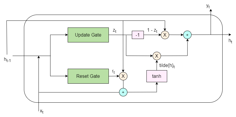
The key idea behind GRUs is to use gating mechanisms to control the flow of information within the network. GRUs have two main gates: the update gate and the reset gate. These gates regulate the amount of information that is retained from the previous time step and the amount of new information that is added at the current time step.
Architectural Components
Figure – GRU architecture
The GRU architecture consists of the following key components:
Update Gate (z):
The update gate determines how much of the previous hidden state should be carried forward to the current time step.
It takes the previous hidden state (ht-1) and the current input (xt) as inputs and produces a value between 0 and 1 for each element in the hidden state.
A value of 0 means completely discard the previous hidden state, while a value of 1 means completely retain it.
The update gate equation is given by:
Here, Wz is the weight matrix for the update gate, ht-1 is the previous hidden state, xt is the current input, bz is the bias term, and σ is the sigmoid activation function.
Reset Gate (r):
The reset gate determines how much of the previous hidden state should be forgotten.
It takes the previous hidden state (ht-1) and the current input (xt) as inputs and produces a value between 0 and 1 for each element in the hidden state.
A value of 0 means completely forget the previous hidden state, while a value of 1 means completely retain it.
The reset gate equation is given by:
Here, Wr is the weight matrix for the reset gate, and br is the bias term.
Candidate Hidden State (h):
The candidate hidden state represents the new information that could potentially be added to the current hidden state.
It is computed based on the current input (xt) and the element-wise product of the reset gate (rt) and the previous hidden state (ht-1).
The candidate hidden state equation is given by:
Here, Wh is the weight matrix for the candidate hidden state, bh is the bias term, and tanh is the hyperbolic tangent activation function.
Hidden State (h):
The hidden state represents the output of the GRU unit at each time step.
It is computed as a linear interpolation between the previous hidden state (ht-1) and the candidate hidden state (h), controlled by the update gate (zt).
The hidden state equation is given by:
Here, zt is the output of the update gate, ht-1 is the previous hidden state, and ht is the candidate hidden state.
Advantages
Simpler architecture: GRUs have fewer parameters and a more streamlined computation process compared to LSTMs, leading to faster training and inference times.
Efficient capturing of long-term dependencies: GRUs effectively capture long-term dependencies in sequential data through gating mechanisms.
Less prone to overfitting: The simpler structure and fewer parameters make GRUs less prone to overfitting compared to LSTMs.
Good performance in various tasks: GRUs have shown competitive performance in tasks such as language modeling, machine translation, and speech recognition.
Limitations
Lack of explicit memory cell: GRUs do not have a separate memory cell like LSTMs, potentially limiting their ability to maintain very long-term dependencies.
Sensitivity to hyperparameters: GRUs can be sensitive to hyperparameter choices, requiring careful tuning for optimal performance.
Limited interpretability: Understanding the learned representations and decision-making process in GRUs can be challenging.
Challenges with very long sequences: GRUs may struggle to capture dependencies in extremely long sequences.
Despite these limitations, GRUs have proven to be a powerful and efficient alternative to LSTMs for modeling sequential data. Their simpler structure and competitive performance have made them a popular choice in various domains, particularly when computational efficiency is a concern.
Researchers and practitioners often experiment with both LSTMs and GRUs to determine which architecture works best for their specific task and dataset. The choice between LSTMs and GRUs depends on factors such as the complexity of the task, the size of the dataset, the available computational resources, and the desired trade-off between performance and simplicity.
In recent years, the field of NLP has witnessed significant advancements, largely driven by the development of the Transformer architecture and its variants, such as BERT (Bidirectional Encoder Representations from Transformers). In this section, we will explore the Transformer architecture, its key components, and how BERT builds upon this foundation to achieve state-of-the-art performance on a wide range of NLP tasks.
The Transformer architecture, introduced by Vaswani et al. in the paper "Attention Is All You Need," has revolutionized the way NLP models process and understand sequential data. Unlike previous architectures, such as RNNs and LSTM networks, the Transformer relies solely on attention mechanisms to capture dependencies between input tokens.
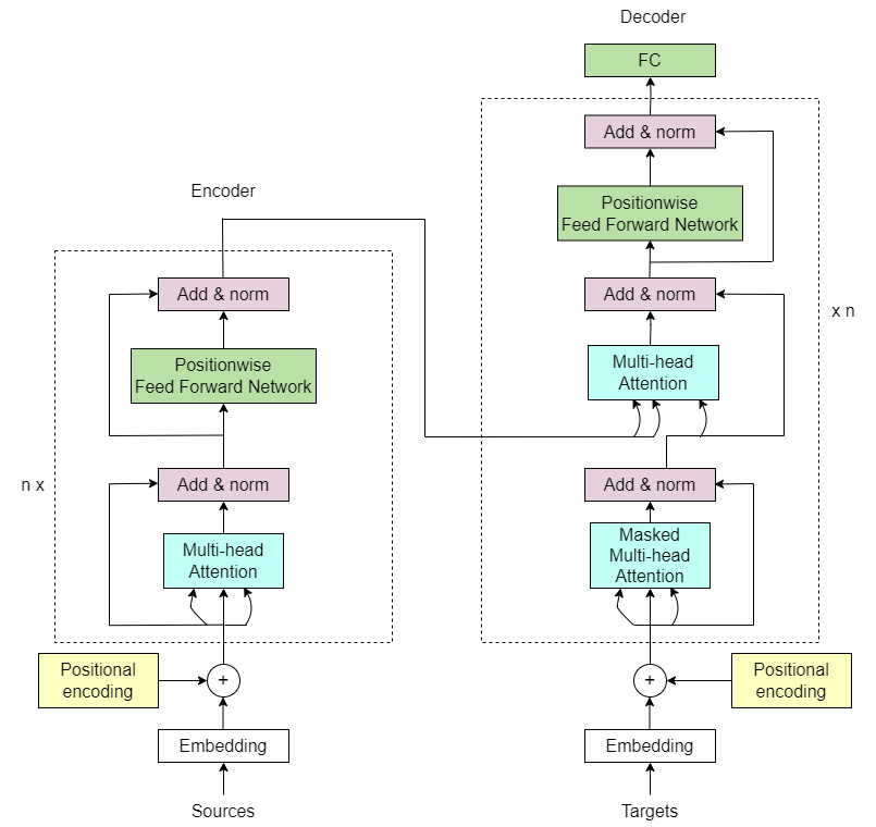
Figure – Transformer architecture
Encoder-Decoder Structure
The Transformer consists of an encoder and a decoder, each composed of a stack of identical layers. The encoder takes the input sequence and generates a contextualized representation, while the decoder generates the output sequence based on the encoder's output and the previously generated tokens.
Multi-Head Attention
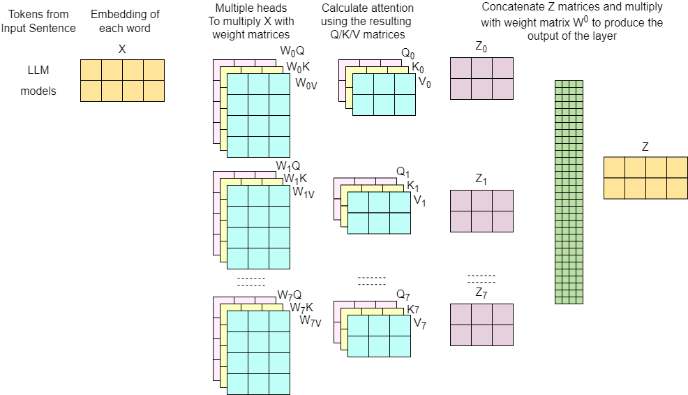
At the core of the Transformer architecture is the multi-head attention mechanism. Multi-head attention allows the model to jointly attend to information from different representation subspaces at different positions. It enables the model to capture complex relationships and dependencies between tokens in the input sequence.
In multi-head attention, the input sequence is projected into multiple query, key, and value vectors. The attention weights are computed by taking the dot product between the query and key vectors, followed by a softmax function. The output is obtained by multiplying the attention weights with the value vectors.
Figure – Multi-Head attention
Position-wise Feed-Forward Networks
In addition to multi-head attention, each layer in the Transformer also includes position-wise feed-forward networks. These networks are applied independently to each position in the sequence and consist of two linear transformations with a ReLU activation in between. The feed-forward networks help the model learn higher-level representations and capture complex patterns in the input.
Positional Encoding
Since the Transformer does not rely on recurrent connections, it needs a way to incorporate positional information into the input representations. This is achieved through positional encoding, where each position in the sequence is assigned a unique vector that encodes its relative position. The positional encodings are added to the input embeddings, allowing the model to capture the order and relative positions of the tokens.
Building upon the Transformer architecture, BERT has become one of the most influential and widely-used models in NLP. BERT is designed to pre-train deep bidirectional representations from unlabeled text by jointly conditioning on both left and right context in all layers.
Figure – BERT architecture
BERT is pre-trained on two unsupervised tasks
Masked Language Modeling (MLM): In this task, a random subset of tokens in the input sequence is masked, and the objective is to predict the original vocabulary ID of the masked word based only on its context. This allows the model to learn bidirectional representations by considering both the left and right context.
Next Sentence Prediction (NSP): In this task, the model is given a pair of sentences and learns to predict whether the second sentence follows the first sentence in the original text. This helps the model understand the relationship between sentences, which is crucial for tasks like question answering and natural language inference.
Input Representation
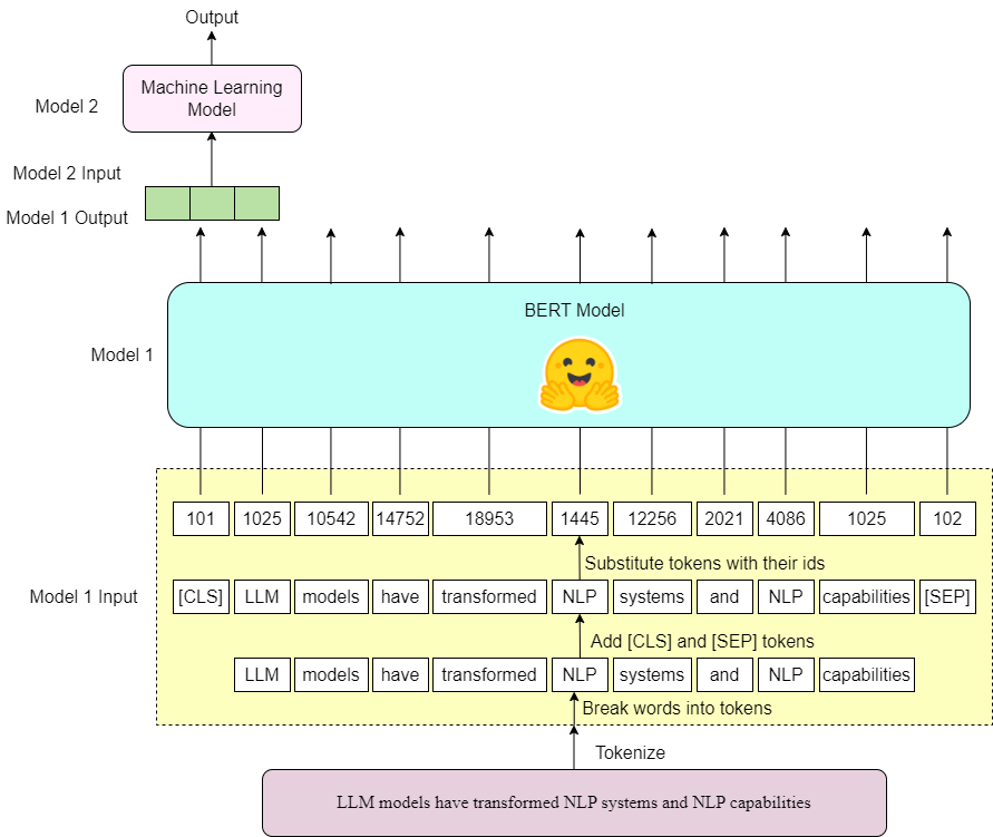
BERT takes a sequence of tokens as input, which can be a single sentence or a pair of sentences separated by a special token ([SEP]). The input representation for each token is constructed by summing the corresponding token embedding, segment embedding, and position embedding.
Fine-tuning
One of the key strengths of BERT is its ability to be fine-tuned for specific downstream tasks with minimal modifications. By adding a task-specific output layer on top of the pre-trained BERT model, it can be adapted to various NLP tasks, such as sentiment analysis, named entity recognition, and question answering.
During fine-tuning, the pre-trained BERT parameters are initialized, and the model is trained on a labeled dataset specific to the downstream task. The model learns to map the input sequences to the desired output format, leveraging the rich representations learned during pre-training.
Advantages and Limitations
BERT has several advantages that have contributed to its success:
Bidirectional representations: BERT's ability to learn from both left and right context allows it to capture more accurate and nuanced representations of words and their relationships.
Unsupervised pre-training: By pre-training on large unlabeled text corpora, BERT can learn general language representations that can be fine-tuned for specific tasks with relatively small labeled datasets.
State-of-the-art performance: BERT has achieved state-of-the-art results on a wide range of NLP benchmarks, demonstrating its effectiveness in capturing contextual information and learning rich representations.
However, BERT also has some limitations:
Computational complexity: BERT has a large number of parameters and requires significant computational resources for pre-training and fine-tuning, which can be a challenge for resource-constrained environments.
Limited sequence length: BERT has a fixed maximum sequence length (typically 512 tokens), which can be a limitation for tasks that require processing longer sequences or documents.
Lack of interpretability: Like many deep learning models, BERT's internal representations and decision-making process can be difficult to interpret, which can be a concern in certain applications where explainability is important.
Despite these limitations, BERT has had a profound impact on the field of NLP and has paved the way for further advancements in language modeling and understanding.
Code:
!pip install transformers
import numpy as np
import pandas as pd
from sklearn.model_selection import train_test_split
from sklearn.svm import SVC
from sklearn.model_selection import cross_val_score
import torch
import transformers as ppb
df = pd.read_csv('/path/train.tsv', delimiter='\t', header=None)
batch_1 = df[:2500]
# For DistilBERT:
model_class, tokenizer_class, pretrained_weights = (ppb.DistilBertModel, ppb.DistilBertTokenizer, 'distilbert-base-uncased')
## Want BERT instead of distilBERT? Uncomment the following line:
#model_class, tokenizer_class, pretrained_weights = (ppb.BertModel, ppb.BertTokenizer, 'bert-base-uncased')
# Load pretrained model/tokenizer
tokenizer = tokenizer_class.from_pretrained(pretrained_weights)
model = model_class.from_pretrained(pretrained_weights)
tokenized = batch_1[0].apply((lambda x: tokenizer.encode(x, add_special_tokens=True)))
max_len = 0
for i in tokenized.values:
if len(i) > max_len:
max_len = len(i)
padded = np.array([i + [0]*(max_len-len(i)) for i in tokenized.values])
attention_mask = np.where(padded != 0, 1, 0)
attention_mask.shape
input_ids = torch.tensor(padded)
attention_mask = torch.tensor(attention_mask)
with torch.no_grad():
last_hidden_states = model(input_ids, attention_mask=attention_mask)
features = last_hidden_states[0][:,0,:].numpy()
labels = batch_1[1]
train_features, test_features, train_labels, test_labels = train_test_split(features, labels)
lr_clf = SVC()
lr_clf.fit(train_features, train_labels)
lr_clf.score(test_features, test_labels)
Description:
The code demonstrates how to use the BERT model for sentiment classification of movie reviews using the Hugging Face Transformers library. The dataset consists of movie reviews labeled as either positive or negative. Here's a step-by-step explanation:
The necessary libraries are imported, including NumPy, pandas, scikit-learn, PyTorch, and the Transformers library.
The movie review dataset is loaded from a TSV file using pandas. In this example, only the first 2500 rows of the dataset are used (stored in batch_1).
The BERT model and tokenizer are loaded using the BertModel and BertTokenizer classes from the Transformers library. The 'bert-base-uncased' pre-trained weights are used.
An attention mask is created to indicate which tokens are actual words (1) and which are padding tokens (0).
The padded input sequences and attention mask are converted to PyTorch tensors.
The BERT model is used to generate hidden state representations for the input sequences. The last hidden states are obtained by passing the input IDs and attention mask to the model.
The features are extracted from the last hidden states by taking the first token's representation (usually the [CLS] token) for each sequence.
The sentiment labels (positive or negative) are obtained from batch_1[1].
A Support Vector Machine (SVM) classifier is initialized and trained on the training features and labels.
If you have any inquiries, feel free to reach out via message or email.














Comments
Nothing yet. Say the first thing.
Sign in to join the conversation.