
Table of Content
2.1 Text Representation Techniques: Bag-of-words, TF-IDF, Word2Vec, GloVe, FastText
2.1.1 Mathematical foundations of text representation techniques
2.1.2 Algorithmic implementation details
2.1.3 Comparative evaluation of different techniques
2.2 Embeddings (ELMo, BERT) and contextual representation
2.2.1 Architecture and design of ELMo and BERT
2.2.2 Pre-Training approaches for contextual embeddings
2.2.3 Fine-tuning contextual embeddings
Written in Collaboration - Special thanks to Manan Thakkar for his valuable contributions to the structure and content of this chapter, shaping it into an informative and accessible resource for understanding text representation techniques.
The ability to understand and generate human language is central to NLP. To achieve this, NLP systems must be able to represent the meaning of language in a way that computers can process. This chapter provides an overview of key techniques for representing text as mathematical vectors, enabling statistical and neural network models to extract semantic information from language data.
We first introduce the bag-of-words model and term frequency-inverse document frequency (TF-IDF), classic approaches that represent text based on word frequencies. Then, we explore neural embedding techniques like Word2Vec, GloVe, and FastText that capture semantic relationships between words. Next, we discuss contextual representation techniques like ELMo and BERT that incorporate the context around words to represent meaning.
By the end of this chapter, you will have strong conceptual and mathematical foundations regarding text representation, enabling you to develop predictive NLP systems. The techniques presented form the basis for contemporary NLP with deep neural networks.
In this chapter, we will cover the following topics:
Text Representation Techniques: Mathematical foundations, algorithms, and evaluation for bag-of-words, TF-IDF, Word2Vec, GloVe, and FastText
Contextualized Embeddings: Architectures, pre-training, and fine-tuning methods for models like ELMo and BERT
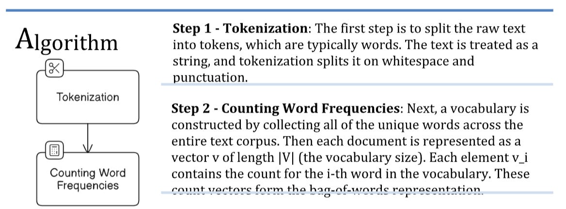
Text representation is a fundamental task in NLP that transforms raw text into vector representations with numerical values that can be readily used by machine learning models. Early techniques like bag-of-words and TF-IDF represented text based on word frequencies, ignoring word order but capturing basic statistical patterns. More recent neural embedding methods like Word2Vec, GloVe, and FastText aim to encode semantic similarity between words into vector representations. In this section, we provide an overview of these major approaches for representing text, outlining the key concepts, algorithms, and evaluation procedures. We begin with a discussion of bag-of-words and TF-IDF, building up intuitions before presenting more complex semantic embedding strategies. By the end, you will have strong foundations regarding how NLP systems numerically represent language for prediction and analysis using vector representations.
The bag-of-words model is one of the earliest and simplest ways to represent text numerically for machine learning. As the name suggests, it treats each document as an unordered collection of words, disregarding grammar and word order entirely. The central idea behind this representation is to capture the basic statistical information about the frequencies of words within a document. Each document is modeled as a multiset or "bag" of its words. The grammar and ordering of the words is ignored, and only the word counts matter.
Concretely, each document is represented as a vector containing the counts for each unique word or token in the vocabulary. This vector encodes the word frequencies but disregards contextual relationships between words. The dimensionality of the vector is equal to the number of unique words across the corpus.
Example:
To illustrate how the bag-of-words model transforms text into numerical vectors, let's walk through a simple example. Consider the following two sentences:
Document 1: “NLP has advanced rapidly in recent years”
Document 2: “LLM models have transformed NLP systems and NLP capabilities”
We first preprocess the sentences by lowercasing, removing stopwords, and lemmatizing to obtain:
Corpus = ['nlp advance rapidly recent years',
'llm model transform nlp systems nlp capabilities']
Looking at all the unique words, our vocabulary is:
['advance', 'capabilities', 'llm', 'model', 'nlp', 'rapidly', 'recent', 'systems', 'transform', 'years']
With this 10-word vocabulary, we can represent each sentence as a 10-dimensional count vector. Element i contains the count of the i-th vocabulary word in that sentence.
For sentence 1, the count of words is as follow:
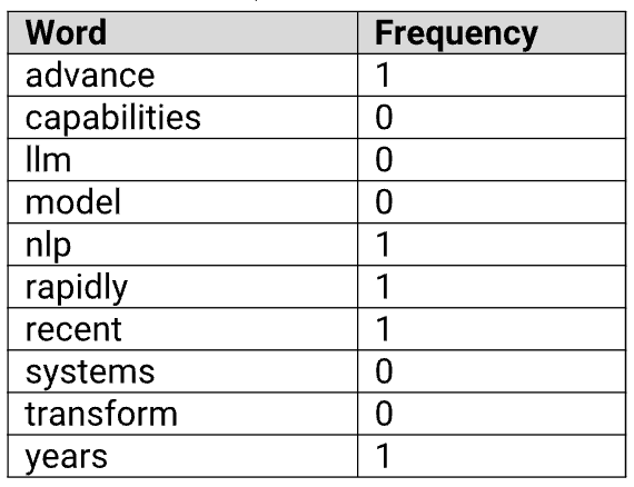
For Sentence 1, the vector is [1, 0, 0, 0, 1, 1, 1, 0, 0, 1], with counts for "nlp", "advance", "rapidly", "recent", and "years".
Now for sentence 2, the scoring would be like
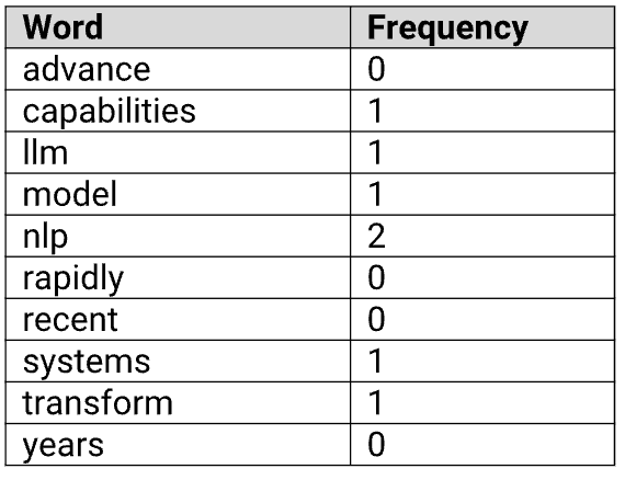
Similarly, the vector for Sentence 2 is [0, 1, 1, 1, 2, 0, 0, 1, 1, 0], with counts for the rest of the vocabulary words.

The approach used in example two is the one that is generally used in the Bag-of-Words technique, the reason being that the datasets used in Machine learning are tremendously large and can contain vocabulary of a few thousand or even millions of words. Hence, preprocessing the text before using bag-of-words is a better way to go.
Advantages
Simplicity: The bag-of-words approach is very simple to understand and implement. Tokenization and counting frequencies are computationally straightforward.
Efficiency: Constructing the vocabulary and transforming documents into count vectors can be done very efficiently with sparse matrix representations. This allows bag-of-words to scale to large datasets.
Effectiveness for classification: Despite its flaws, bag-of-words works reasonably well for document classification tasks. The word frequencies provide enough statistical signal for simple categorical predictions.
Limitations
Lacks word order: Completely discarding word order is a major limitation. The model cannot differentiate "dogs bite men" from "men bite dogs" as the counts are identical. Position and sequence are lost.
Ignores context: Counts are aggregated globally across the document, ignoring local context. The distributions of words in different sections of text are not captured.
No phrase modeling: Bag-of-words looks at single words only, not phrases. So "New York Times" is treated as separate unrelated words.
High dimensionality: The vocabulary size directly determines the number of dimensions. Real-world datasets can easily have vocabularies in the millions, leading to extremely high-dimensional representations. This causes sparsity and statistical issues.
No semantics: Synonyms like "smart" and "intelligent" are treated as unrelated. Semantic meaning is lost without representations of word-word relations.
Rare words: Words not seen during training are ignored entirely. But rare or new words can be highly informative, such as technical terms or neologisms.
Here is sample Python code to generate a bag-of-words representation:
import numpy as np
corpus = [' nlp advance rapidly recent years ',
' llm model transform nlp systems nlp capabilities ']
vocab = ['advance', 'capabilities', 'llm', 'model', 'nlp', 'rapidly', 'recent', 'systems', 'transform', 'years']
position = {}
for i, token in enumerate(vocab):
position[token] = i
print(position)
bow_matrix = np.zeros((len(preprocessed_corpus), len(vocab)))
for i, preprocessed_sentence in enumerate(preprocessed_corpus):
for token in preprocessed_sentence.split():
bow_matrix[i][position[token]] = bow_matrix[i][position[token]] + 1
bow_matrix
OUTPUT:
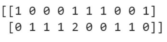
This code snippet demonstrates how to construct a bag-of-words representation matrix from a preprocessed text corpus.
First, the pre-processed corpus and vocabulary as a list of all unique words extracted from the corpus using word tokenizer are defined. Then, a position dictionary is created to map each word to an index value.
Next, a blank bag-of-words matrix is initialized with shape (num_documents, vocabulary_size), to store the word counts for each document. We loop through each preprocessed sentence in the corpus, splitting into words. For each word, we increment the count at the corresponding vocabulary index in the bow_matrix for that document.
By the end, bow_matrix will contain the bag-of-words representation where each row is the word count vector for a document. This matrix encodes the word frequencies but lacks word order and semantics.
This code demonstrates an efficient and vectorized approach to generate bag-of-words representations from text corpora before feeding into machine learning models. The simple counts capture basic statistics but not linguistic meaning.
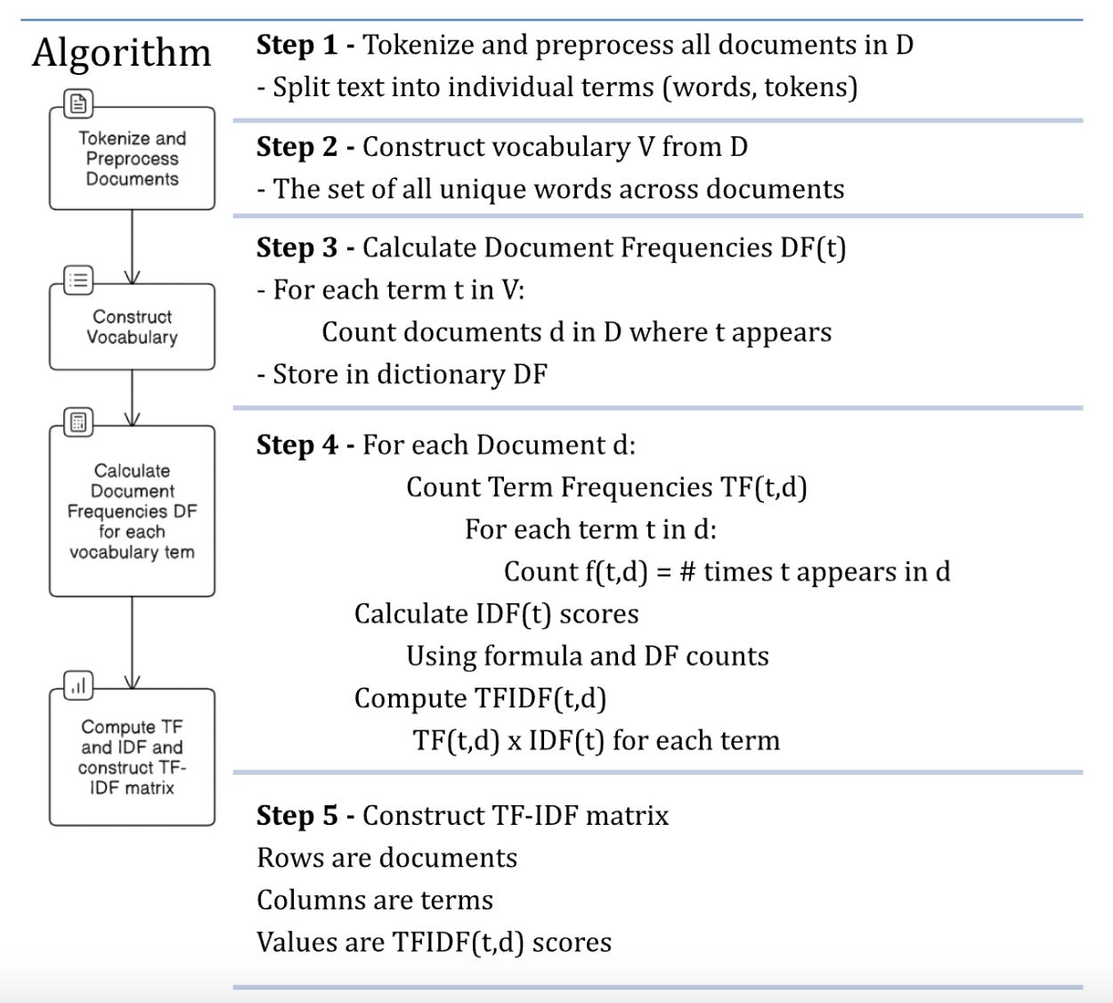
The standard bag-of-words representation that underpins many text analysis models utilizes raw term frequencies (TF) as the primary feature values. However, frequency alone does not always capture relevance. Extremely common words can appear with high regularity just by chance, overwhelming the signal from rarer but more informative keywords.
To counteract this tendency, the TF-IDF scheme introduces a second weighting factor called inverse document frequency (IDF). This rebalances weights so that ubiquitous terms are scaled down and distinctive salient terms are scaled up. Specifically, IDF measures how common or unique a word is across the entire document corpus by taking the logarithm of the inverse fraction of documents containing that word. Values are higher for words occurring in fewer documents, tapering for broadly common words.
Multiplying the TF and IDF assigns the highest scores to words that strike an optimal balance - frequent enough locally to be relevant for a document, but globally rare enough to uniquely describe a document's meaning. This amplifies keywords that characterize document content rather than broadly useless words.
For example, “phone” may appear often in a cell phone manual, but so do generic terms like "settings" and "menu" across many documents. The IDF downweights these widely common words so that meaningful keywords like “phone” rise to the top.
The TF-IDF score for a term in a document is calculated as the product of its TF and IDF. Here are the equations for TF and IDF, and the overall TF-IDF:
Term-Frequency (TF):

Inverse Document Frequency (IDF):

TF-IDF:

Example:
To illustrate how the bag-of-words model transforms text into numerical vectors, let's walk through a simple example. Consider the following two sentences:
Document 1: “NLP has advanced rapidly in recent years”
Document 2: “LLM models have transformed NLP systems and NLP capabilities”
Example:
To illustrate TF-IDF vectorization, consider the same pre-processed statements as our corpus:
Document 1: “nlp advance rapidly recent years”
Document 2: “llm model transform nlp systems nlp capabilities”
The full set of unique words across both documents forms the vocabulary V:
V = {nlp, advance, rapidly, recent, years, llm, model, transform, systems, capabilities}
Total Vocabulary Size = 10 terms
Calculate Term Frequencies (TF)
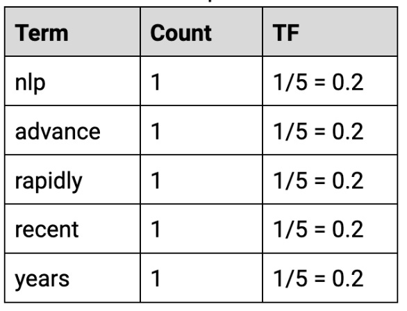
Doc 1:
Number of words/terms = 5 terms
Calculate TF per term as: Number of occurrences / Total terms
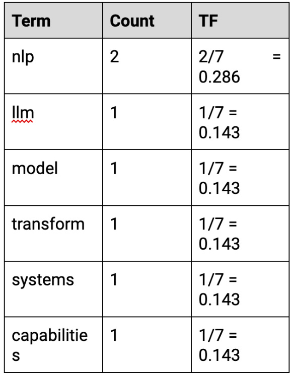
Doc 2:
Number of words/terms = 7 terms
Repeat TF calculation:
Calculate the Document Frequency (DF) and Inverse Document Frequencies (IDF)
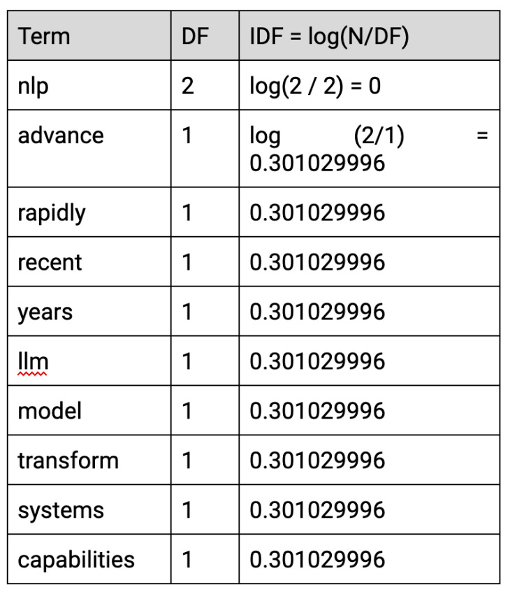
Calculate TF-IDF Scores
TF-IDF = TF * IDF
Showing vector scores:
Doc 1: [0, 0.06020600, 0.06020600, 0.06020600, 0.06020600, 0, 0, 0, 0, 0]
Doc 2: [0, 0, 0, 0, 0, 0.0427665, 0.0427665, 0.0427665, 0.0427665, 0.0427665]
Advantages
Measures Term Relevance: TF-IDF effectively identifies terms that are relevant in a particular document compared to the entire corpus based on frequency contrasts. High scores mean a term captures key topical content.
Handles Large Corpora: The TF-IDF formulation scales to huge text collections with sparse matrix representations, making it suitable for big data scenarios. Memory-efficient implementations are feasible.
Reduces Impact of Common Terms: TF-IDF automatically downweights ubiquitous stop words that lack informational value, preventing domination by generic frequent terms.
Applicable for Many Tasks: TF-IDF creates descriptive feature representations that provide good performance across applications like search, classification, clustering, and more.
Interpretable Scores: The TF-IDF scores assign direct quantitative assessments of term importance. This enables qualitative analysis of a document's key themes.
Limitations
No Semantic Analysis: TF-IDF treats semantic relationships between words superficially. Synonyms and related terms are viewed as independent.
Assumption of Term Independence: The formulation assumes words occurring in a document are independent, whereas natural language contains more complex linguistic relationships.
High Dimensionality: The vocabulary size can easily reach millions, leading to very wide, sparse matrices that create statistical issues.
Lacks Word Order Modeling: All terms are represented equally regardless of sequence, discarding order dependence and syntactic context.
Hyper parameters Performance Impact: Stopword removal and smoothing schemes for IDF can significantly sway overall results. TF-IDF requires careful tuning.
Here is sample Python code to generate a TF-IDF vector representation:
import numpy as np
corpus = [' nlp advance rapidly recent years ',
' llm model transform nlp systems nlp capabilities ']
vectorizer = TfidfVectorizer()
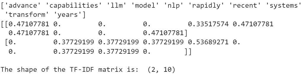
tf_idf_matrix = vectorizer.fit_transform(preprocessed_corpus)
print(vectorizer.get_feature_names_out())
print(tf_idf_matrix.toarray())
print("\nThe shape of the TF-IDF matrix is: ", tf_idf_matrix.shape)
OUTPUT:
Word2Vec is a popular technique for learning word embeddings, which are dense vector representations of words in a continuous vector space. It was introduced by Tomas Mikolov and his colleagues at Google in 2013. The main idea behind Word2Vec is to capture semantic and syntactic relationships between words based on their co-occurrence patterns in a large corpus of text.
The Need for Word2Vec:
Traditional bag-of-words and TF-IDF representations have several limitations. They treat words as discrete and independent entities, ignoring their semantic relationships and context. This makes it difficult to capture the meaning and similarity between words. Word2Vec addresses these limitations by learning dense vector representations that capture the semantic and syntactic relationships between words.
Techniques in Word2Vec:
Word2Vec consists of two main techniques for learning word embeddings:
1.Continuous Bag-of-Words (CBOW):
In CBOW, the model predicts the target word based on its surrounding context words.
The input to the model is the context words (e.g., a window of words around the target word), and the output is the target word.
The objective is to maximize the probability of predicting the target word given its context.
CBOW is computationally efficient and works well with small datasets.
2.Skip-Gram:
In Skip-Gram, the model predicts the surrounding context words given a target word.
The input to the model is the target word, and the output is the context words.
The objective is to maximize the probability of predicting the context words given the target word.
Skip-Gram is more effective in capturing rare words and performs better with larger datasets.
Importance of Word2Vec:
Word2Vec has revolutionized the field of NLP by providing a powerful way to represent words as dense vectors. Its importance can be highlighted through the following points:
Semantic Relationships: Word2Vec captures semantic relationships between words. Words with similar meanings are mapped to nearby points in the vector space. This allows for measuring the semantic similarity between words using cosine similarity or Euclidean distance.
Analogy Reasoning: Word2Vec enables analogy reasoning through simple vector arithmetic. For example, the analogy "king - man + woman = queen" can be solved by performing vector operations on the corresponding word embeddings.
Transfer Learning: Word embeddings learned using Word2Vec can be used as pre-trained features for various downstream NLP tasks, such as sentiment analysis, named entity recognition, and text classification. This transfer learning approach has shown significant improvements in performance.
Dimensionality Reduction: Word2Vec reduces the dimensionality of word representations compared to one-hot encoding or TF-IDF. This makes it more computationally efficient and allows for better generalization.
Language Model Pre-training: Word2Vec has paved the way for more advanced language model pre-training techniques, such as GloVe, FastText, and contextual embedding like ELMo and BERT. These models build upon the ideas of Word2Vec to capture even richer linguistic information.
Skip-Gram:
The Skip-Gram model is a powerful technique for learning dense vector representations of words, known as word embeddings. It aims to predict the surrounding context words given a target word, based on the idea that words occurring in similar contexts tend to have similar meanings.
To understand how the Skip-Gram model works, let's consider an example sentence:
"NLP has advanced rapidly with the rise of LLM models."
In the Skip-Gram model, we choose a target word and aim to predict its surrounding context words within a specified window size. Let's consider the target word "LLM" and a window size of 2.
Target word: "LLM"
Context words: "the", "rise", "of", "models"
The Skip-Gram model will generate pairs of (target word, context word) as training examples:
(LLM, the)
(LLM, rise)
(LLM, of)
(LLM, models)
These pairs are used as input to a neural network. The input to the network is a one-hot encoded vector representing the target word, and the output is a one-hot encoded vector representing the context word. The objective of the model is to maximize the probability of predicting the context words given the target word. Let's explore these components step by step, using the example sentence: "NLP has advanced rapidly with the rise of LLM models."
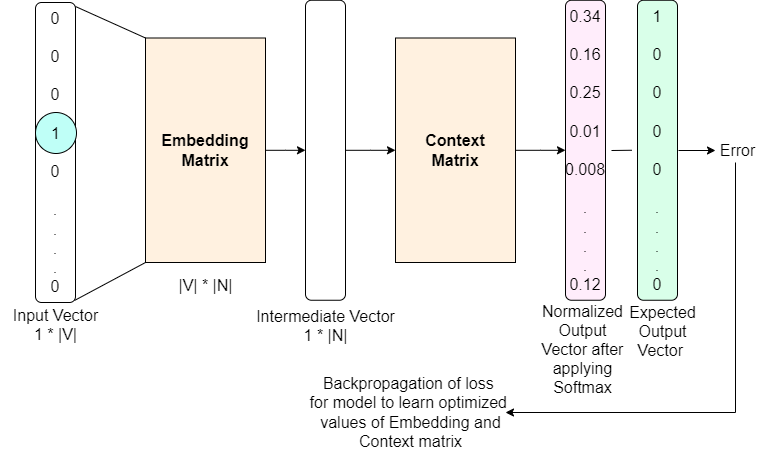
Figure 2.1 – Architectural diagram of Skip-Gram model
Step 1: Vocabulary and One-Hot Encoding
Define the vocabulary V, which is the set of unique words in the corpus.
Assign a unique index to each word in the vocabulary.
Represent the input and output words using one-hot encoding.
The one-hot encoded vector has a single 1 at the index corresponding to the word and 0s everywhere else.
The size of the one-hot encoded vector is equal to the vocabulary size |V|.
Example:
Let's say our vocabulary V consists of the following words: ["NLP", "has", "advanced", "rapidly", "with", "the", "rise", "of", "LLM", "models"].
The one-hot encoded vector for the word "NLP" would be: [1, 0, 0, 0, 0, 0, 0, 0, 0, 0], where the vector has size |V| = 10.
Step 2: Input Layer
The input to the Skip-Gram model is a one-hot encoded vector representing the target word.
The input layer has |V| neurons, each representing a word in the vocabulary.
The input layer is fully connected to the hidden layer.
Example:
If the target word is "LLM", the input to the Skip-Gram model would be a one-hot encoded vector of size |V| = 10, with a 1 at the index corresponding to "LLM" and 0s everywhere else.
Step 3: Embedding Matrix
The embedding matrix is a matrix of size |V| × N, where N is the dimensionality of the word embeddings.
Each row of the embedding matrix represents the word embedding for a specific word in the vocabulary.
The embedding matrix is denoted as Matrix W in the diagram.
The initialization of the embedding matrix is an important consideration in the Skip-Gram model. The choice of initialization can impact the model's performance and convergence during training. There are several common approaches to initializing the embedding matrix such as: Random Initialization, Pre-trained Embeddings, Xavier Initialization, and He Initialization.
Example:
If we choose an embedding dimensionality of N = 5, the embedding matrix would have size |V| × N = 10 × 5.
Step 4: Hidden Layer
The hidden layer is obtained by multiplying the one-hot encoded input vector x of size |V| × 1 with the embedding matrix W of size |V| × N.
The resulting hidden layer h is a vector of size 1 × N, representing the word embedding of the target word.
Example:
Given the one-hot encoded input vector x for the target word "LLM" and the embedding matrix W, the hidden layer h would be computed as: h = x × W, resulting in a vector of size 1 × N.
Step 5: Context Matrix
The context matrix is a matrix of size N × |V|, denoted as Matrix W' in the diagram.
It maps the word embeddings from the hidden layer to the output layer.
Step 6: Output Layer
The output layer predicts the probabilities of each word in the vocabulary being a context word for the target word.
It is obtained by multiplying the hidden layer h of size 1 × N with the context matrix W' of size N × |V|.
The resulting output is a vector of size 1 × |V|, representing the probabilities of each word being a context word.
Step 7: Output Softmax
The output vector undergoes a softmax activation function to convert the scores into probabilities.
The softmax function normalizes the output vector, ensuring that the probabilities sum up to 1.
Example:
For the target word "LLM", the output vector after the softmax function would represent the probabilities of each word in the vocabulary being a context word. The words with higher probabilities, such as "models", "advanced", and "NLP", would be considered more likely to appear in the context of "LLM".
The Skip-Gram model is trained using techniques like stochastic gradient descent to optimize the embedding matrix W and the context matrix W'. The objective is to maximize the probability of predicting the correct context words given the target word.
Code:
import numpy as np
from collections import defaultdict
class Word2Vec:
def __init__(self, corpus, window_size, embedding_size, learning_rate, epochs):
self.corpus = corpus
self.window_size = window_size
self.embedding_size = embedding_size
self.learning_rate = learning_rate
self.epochs = epochs
self.word_to_id, self.id_to_word = self.create_vocabulary()
self.word_counts = self.count_words()
self.embeddings = self.initialize_embeddings()
self.context_weights = self.initialize_context_weights()
def create_vocabulary(self):
words = set(self.corpus)
word_to_id = {word: i for i, word in enumerate(words)}
id_to_word = {i: word for i, word in enumerate(words)}
return word_to_id, id_to_word
def count_words(self):
word_counts = defaultdict(int)
for word in self.corpus:
word_counts[word] += 1
return word_counts
def initialize_embeddings(self):
vocab_size = len(self.word_to_id)
embeddings = np.random.uniform(-0.5, 0.5, (vocab_size, self.embedding_size))
return embeddings
def initialize_context_weights(self):
vocab_size = len(self.word_to_id)
context_weights = np.random.uniform(-0.5, 0.5, (self.embedding_size, vocab_size))
return context_weights
def softmax(self, x):
exp_x = np.exp(x - np.max(x))
return exp_x / np.sum(exp_x)
def train(self):
for epoch in range(self.epochs):
loss = 0
for i in range(len(self.corpus)):
center_word = self.corpus[i]
center_word_id = self.word_to_id[center_word]
context_words = self.get_context_words(i)
for context_word in context_words:
context_word_id = self.word_to_id[context_word]
# Forward pass
hidden_layer = self.embeddings[center_word_id]
output_layer = np.dot(hidden_layer, self.context_weights)
output_probs = self.softmax(output_layer)
# Calculate error and update weights
error = output_probs.copy()
error[context_word_id] -= 1
# Backpropagation
grad_context_weights = np.outer(hidden_layer, error)
grad_embeddings = np.dot(error, self.context_weights.T)
# Update weights
self.context_weights -= self.learning_rate * grad_context_weights
self.embeddings[center_word_id] -= self.learning_rate * grad_embeddings
loss += -np.log(output_probs[context_word_id])
print(f"Epoch: {epoch+1}, Loss: {loss}")
def get_context_words(self, i):
start = max(0, i - self.window_size)
end = min(len(self.corpus), i + self.window_size + 1)
context_words = self.corpus[start:i] + self.corpus[i+1:end]
return context_words
# Example usage
corpus = ["NLP", "has", "advanced", "rapidly", "with", "the", "rise", "of", "LLM", "models"]
window_size = 2
embedding_size = 50
learning_rate = 0.01
epochs = 10
word2vec = Word2Vec(corpus, window_size, embedding_size, learning_rate, epochs)
word2vec.train()
# Get the vector representations of the context words
center_word = "rise"
center_word_id = word2vec.word_to_id[center_word]
context_words = word2vec.get_context_words(word2vec.corpus.index(center_word))
context_vectors = []
for context_word in context_words:
context_word_id = word2vec.word_to_id[context_word]
context_vector = word2vec.context_weights[:, context_word_id]
context_vectors.append(context_vector)
print(f"Context words for '{center_word}': {context_words}")
print(f"Vector representations of the context words:")
for i, context_vector in enumerate(context_vectors):
print(f"{context_words[i]}: {context_vector}")
This code implements the Word2Vec model using the Skip-Gram architecture from scratch. Here's a breakdown of the code:
The Word2Vec class is defined with the following attributes:
corpus: The input corpus of words.
window_size: The size of the context window.
embedding_size: The dimensionality of the word embeddings.
learning_rate: The learning rate for weight updates.
epochs: The number of training epochs.
The create_vocabulary method creates a mapping between words and their corresponding IDs and vice versa.
The count_words method counts the frequency of each word in the corpus.
The initialize_embeddings method initializes the word embeddings matrix with random values.
The initialize_context_weights method initializes the context weights matrix with random values.
The softmax method applies the softmax activation function to the output layer.
The train method trains the Word2Vec model using the Skip-Gram architecture. It iterates over each word in the corpus, identifies the context words within the specified window, and performs forward and backward propagation to update the embeddings and context weights.
The get_context_words method retrieves the context words for a given center word.
Word2Vec using pre-trained model
One of the advantages of Word2Vec is the availability of pre-trained models that have already been trained on large datasets. These pre-trained models can be readily used for various NLP tasks without the need for training from scratch. One popular library that provides pre-trained Word2Vec models and easy-to-use functionality is Gensim.
Here's an explanation of how to use pre-trained Word2Vec models with Gensim, along with code examples:
Installation: To use Gensim, you first need to install it. You can install Gensim using pip:
pip install gensim
Gensim is a popular open-source library for unsupervised topic modeling and NLP, with a focus on handling large text collections. It provides efficient and scalable implementations of various algorithms, including Word2Vec, for learning word embeddings from text data. Gensim is designed to be easy to use and integrate with other libraries in the Python ecosystem.
Loading a pre-trained Model: Gensim provides several pre-trained Word2Vec models that you can easily load. One commonly used model is the Google News model, which was trained on a large corpus of Google News articles. The Google News Word2Vec model consists of 300-dimensional word vectors for approximately 3 million words and phrases. Here's an example of how to load the Google News model:
from gensim.models import KeyedVectors
# Load the pre-trained Google News model
model = KeyedVectors.load_word2vec_format(' path/to/GoogleNews-vectors-negative300.bin.gz ', binary=True)
Accessing Word Vectors: Once the pre-trained model is loaded, you can access the word vectors using the [] operator. Here's an example:
# Get the vector representation of a word
vector = model['natural']
print(vector)
This will retrieve the vector representation of the word “natural” from the pre-trained model.
Word Similarity: Word2Vec embeddings capture semantic similarity between words. You can use the similarity() method to calculate the cosine similarity between two words:
# Calculate similarity between words
similarity = model.similarity(‘NLP’, ‘LLM’)
print(similarity)
Finding Similar Words: You can find the most similar words to a given word using the most_similar() method:
# Find the most similar words
similar_words = model.most_similar('LLM', topn=5)
print(similar_words)
Analogy Reasoning: Word2Vec embeddings can also be used for analogy reasoning, where you can find the word that completes an analogy. The most_similar() method can be used with positive and negative words:
# Perform analogy reasoning
result = model.most_similar(positive=['Natural', 'Language'], negative=['Processing'], topn=1)
print(result)
This will find the word that completes the analogy “king - man + woman = ?” based on the learned word embeddings.
FastText is an open-source library developed by Facebook AI Research (FAIR) for efficient learning of word embeddings and text classification. It is an extension of the Word2Vec model, designed to address some of its limitations and improve upon its performance. FastText has gained popularity due to its ability to handle large-scale datasets efficiently and its effectiveness in capturing subword information.
Word2Vec has been a groundbreaking model for learning word embeddings, but it has certain limitations. One of the main drawbacks of Word2Vec is its inability to handle out-of-vocabulary (OOV) words. When Word2Vec encounters a word that was not present in the training data, it cannot provide a meaningful representation for that word. This is problematic when dealing with morphologically rich languages or specialized domains with rare or novel words.
FastText addresses this limitation by introducing the concept of subword embeddings. Instead of learning embeddings only for whole words, FastText breaks words into smaller subword units, such as character n-grams. By representing words as a combination of these subword embeddings, FastText can generate embeddings for OOV words by leveraging the information from their subword components.
FastText's ability to represent words as character n-grams and incorporate subword information sets it apart from other word embedding models like Word2Vec. Let's illustrate this with an example using the sentence we've been working with throughout the chapter:
"LLM models have transformed NLP systems and NLP capabilities."
In the Word2Vec model, each word in this sentence would be treated as a separate entity, and the model would learn embeddings for each word based on its context. However, FastText takes a different approach by breaking down each word into character n-grams.
Let's consider the word "transformed" and represent it using character trigrams (n = 3):
<tra, ran, ans, nsf, sfo, for, orm, rme, med, ed>
FastText would also include the entire word as a separate token:
<tra, ran, ans, nsf, sfo, for, orm, rme, med, ed> and <transformed>
By representing words as character n-grams, FastText captures the morphological and subword information within the words. This is particularly advantageous in several scenarios:
Importance of FastText:
Handling OOV Words: In the given example, let's say the word "transformational" was not present in the training data. Word2Vec would treat it as an unknown word and assign a random or default embedding. However, FastText can generate an embedding for "transformational" by leveraging the subword information it learned from similar words like "transformed" and "transformation".
FastText would break down "transformational" into character n-grams: <tra, ran, ans, nsf, sfo, for, orm, rma, mat, ati, tio, ion, ona, nal, al> By utilizing the learned embeddings for these subword components, FastText can generate a meaningful representation for the OOV word "transformational".
Capturing Morphological Relationships: FastText's subword-based approach allows it to capture morphological relationships between words. In the example sentence, the words "transformed" and "capabilities" share common subword patterns:
“transformed”:
<tra, ran, ans, nsf, sfo, for, orm, rme, med, ed>“capabilities”:
<cap, apa, pab, abi, bil, ili, lit, iti, tie, ies, es>
By recognizing these shared subword components, FastText can understand the morphological similarity between these words and learn similar embeddings for them. This is particularly useful in languages with rich morphology, where words can have multiple inflected forms.
Efficient Representation and Computation: FastText's character n-gram representation allows for efficient storage and computation of word embeddings. Instead of learning separate embeddings for each word, FastText learns embeddings for the subword components. This reduces the number of parameters to be learned and allows for faster training and inference. In the example sentence, FastText would learn embeddings for the character n-grams and the entire words. During inference, the embedding for a word like "transformed" would be computed by combining the embeddings of its subword components, which is computationally efficient compared to storing and retrieving embeddings for every possible word.
Other important points about FastText are:
Text Classification: In addition to learning word embeddings, FastText also provides a simple and efficient method for text classification. It represents text as a bag of word embeddings and uses a linear classifier to predict the class labels. FastText's text classification approach has shown competitive performance compared to more complex deep learning models, especially when dealing with large datasets and multiple classes.
Multilingual Support: FastText has been trained on a wide range of languages and has pre-trained models available for many languages. This multilingual support allows users to easily apply FastText to various language-specific tasks and benefit from the learned embeddings across different languages.
Integration and Extensibility: FastText is open-source and designed to be easily integrated into existing software systems. It provides a simple and intuitive API for training and using word embeddings. FastText can also be extended and customized to suit specific requirements, making it a flexible tool for researchers and practitioners.
Code:
from gensim.models import FastText
# Training data
sentences = [
"LLM models have transformed NLP systems and NLP capabilities.",
"The development of LLM models has revolutionized the field of NLP.",
"FastText is an efficient library for learning word embeddings.",
"FastText captures subword information and handles out-of-vocabulary words.",
]
# Train FastText model
model = FastText(sentences, vector_size=100, window=5, min_count=1, workers=4)
# Get the vocabulary
vocabulary = list(model.wv.key_to_index.keys())
print("Vocabulary:", vocabulary)
# Get the word vector for a word
word = "NLP"
vector = model.wv[word]
print(f"Vector for '{word}': {vector}")
# Find most similar words
similar_words = model.wv.most_similar(word, topn=5)
print(f"Most similar words to '{word}':")
for similar_word, similarity in similar_words:
print(f"- {similar_word}: {similarity}")
# Find similarity between words
word1 = "LLM"
word2 = "NLP"
similarity = model.wv.similarity(word1, word2)
print(f"Similarity between '{word1}' and '{word2}': {similarity}")
# Handle out-of-vocabulary words
oov_word = "transformational"
oov_vector = model.wv[oov_word]
print(f"Vector for OOV word '{oov_word}': {oov_vector}")
Description:
Now, let's go through the detailed description to understand the code:
We start by importing the FastText class from the gensim.models module. Gensim is a popular library for topic modeling and word embeddings.
We define our training data as a list of sentences. In this example, we have a small dataset related to LLM models and NLP.
We create an instance of the FastText model and train it on the provided sentences. The vector_size parameter specifies the dimensionality of the word vectors, window determines the context window size, min_count sets the minimum frequency threshold for words to be included in the vocabulary, and workers specifies the number of worker threads to use during training.
After training, we can access the vocabulary of the model using model.wv.key_to_index.keys(). We print the vocabulary to see the unique words in our dataset.
To get the word vector for a specific word, we use model.wv[word]. In this example, we retrieve the vector for the word "NLP" and print it.
We can find the most similar words to a given word using model.wv.most_similar(). We specify the word of interest and the number of top similar words to retrieve (topn). The method returns a list of tuples containing the similar words and their similarity scores. We print the most similar words to "NLP".
To calculate the similarity between two words, we use model.wv.similarity(). We provide the two words, "LLM" and "NLP", and print their cosine similarity score.
One of the advantages of FastText is its ability to handle out-of-vocabulary (OOV) words. We demonstrate this by trying to retrieve the vector for the word "transformational", which is not present in our training data. FastText can generate a vector for OOV words by leveraging the subword information learned during training.
GloVe (Global Vectors for Word Representation) is an unsupervised learning algorithm for obtaining vector representations for words. It was introduced by Pennington et al. in 2014 as an improvement over existing word embedding techniques like Word2Vec and FastText. GloVe aims to capture both the global statistics of word co-occurrences in a corpus and the local context information.
Previous word embedding methods, such as Word2Vec and FastText, have shown success in capturing semantic and syntactic relationships between words. However, these methods primarily rely on local context information, considering only the words within a fixed window size. They do not explicitly take into account the global co-occurrence statistics of words across the entire corpus.
GloVe addresses this limitation by incorporating both local and global information in the learning process. It leverages the global word-word co-occurrence matrix to capture the overall statistical patterns in the corpus. By doing so, GloVe aims to learn word vectors that better capture the semantic relationships between words.
Importance of GloVe:
Capturing Global Co-occurrence Statistics: GloVe leverages the global word-word co-occurrence matrix to capture overall semantic patterns and relationships between words, considering their broader context and associations.
Efficient Training: GloVe's weighted least squares objective function enables efficient training of word vectors, even on large datasets, making it scalable for real-world applications.
Improved Word Similarity and Analogy Performance: GloVe learns word vectors that effectively reflect semantic relationships, outperforming other methods on benchmark datasets for word similarity and analogy tasks.
Interpretation of Vector Dimensions: GloVe word vectors exhibit interpretable dimensions that can capture specific semantic concepts, such as gender, sentiment, or part-of-speech information.
Integration with Downstream Tasks: GloVe word vectors can be easily integrated into various downstream NLP tasks, serving as input features to enhance performance and generalization capabilities of machine learning models.
Now that we have discussed the concept of GloVe and its importance in capturing both local and global word relationships, let's dive into the technical details of how GloVe learns word vectors using the co-occurrence information.
The core idea behind GloVe is to minimize the difference between the dot product of word vectors and the logarithm of their co-occurrence probabilities. This is achieved through the following objective function:

Where,
V is the vocabulary size,
Xij is the number of times word,
i appears in the context of word j,
fXij is a weighting function,
wi and wj are the word vectors, and
bi and bj are the bias terms.
To illustrate the process of learning GloVe word vectors, let's walk through a step-by-step example using the sentence: "LLM models have transformed NLP systems and NLP capabilities." We'll use a context window size of 4 for this example.
Step 1: Preprocess the text data
Tokenize the text into words
Remove punctuation and convert to lowercase
Create a vocabulary of unique words
Preprocessed: ["llm", "models", "have", "transformed", "nlp", "systems", "and", "nlp", "capabilities"]
Vocabulary: ["llm", "models", "have", "transformed", "nlp", "systems", "and", "capabilities"]
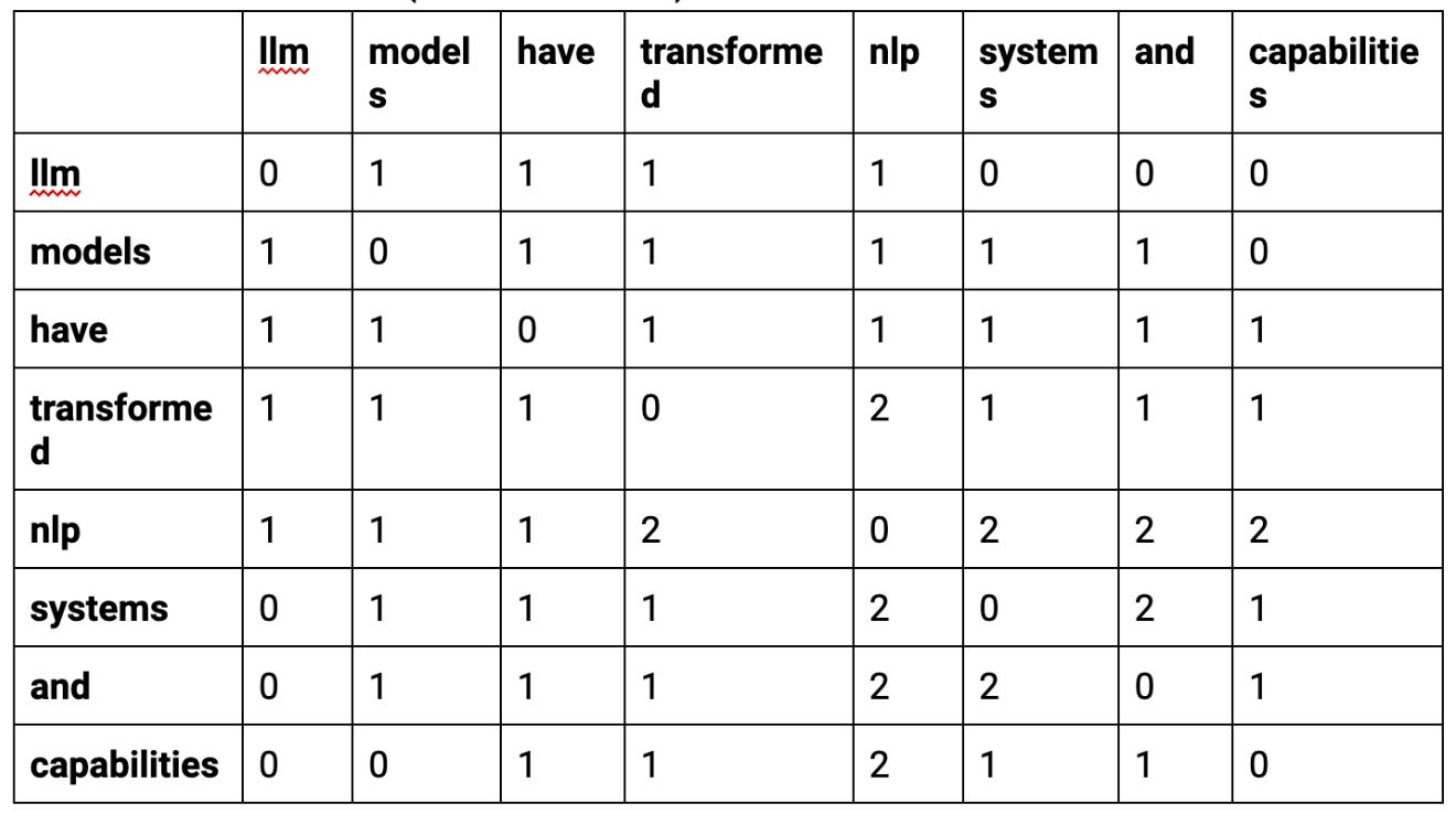
Step 2: Construct the co-occurrence matrix
Define a context window size (in this case, 4)
Iterate through the preprocessed text and count the co-occurrences of word pairs within the context window
Create a symmetric co-occurrence matrix X of size V * V, where V is the vocabulary size
Co-occurrence matrix X (window size = 4):
Step 3: Define the weighting function fXij
Choose a weighting function to assign lower weights to rare and frequent co-occurrences
Common choice: fXij=min1, Xij / xmax
Where, xmax is a threshold and is a parameter (e.g., 0.75)
Assuming xmax = 100 and = 0.75, the weighted co-occurrence matrix fXij remains the same as the co-occurrence matrix X in this example.
Step 4: Initialize word vectors and biases
Randomly initialize word vectors wi and wj of dimension d (e.g., 100) for each word in the vocabulary
Initialize bias terms bi and bj to zero
Step 5: Train the GloVe model
Define the number of training epochs and learning rate
Iterate through each non-zero entry in the weighted co-occurrence matrix $f(X_{ij})$
For each entry (i, j):
Compute the dot product of word vectors: wiT wj
Compute the error term: eij=wiT wj+ bi+ bj -log Xij
Update the word vectors and biases using gradient descent:
wiwi- η.eij.wjwjwj- η.eij.wibibi- η.eijbjbj- η.eij
Repeat for the specified number of epochs
Assuming a learning rate of 0.01 and 50 training epochs, the GloVe model will learn the word vectors wi and wj that capture the semantic relationships between words based on their co-occurrence patterns.
Step 6: Evaluate the learned word vectors
Compute the cosine similarity between word vectors to find similar words
Perform word analogy tasks using vector arithmetic
Use the learned word vectors as features for downstream NLP tasks
After training, the cosine similarity between the word vectors of "nlp" and "capabilities" might be high (e.g., 0.85), indicating their semantic relatedness. Word analogy tasks can also be performed, such as "nlp" - "systems" + "models" ≈ "deep learning".
The learned GloVe word vectors can be used for various NLP applications, such as text classification, sentiment analysis, and information retrieval, as they capture meaningful semantic relationships between words based on their global co-occurrence statistics.
Code:
import numpy as np
from sklearn.metrics.pairwise import cosine_similarity
def create_cooccurrence_matrix(corpus, vocab_size, window_size):
cooccurrence_matrix = np.zeros((vocab_size, vocab_size))
for i in range(len(corpus)):
for j in range(max(0, i - window_size), min(len(corpus), i + window_size + 1)):
if i != j:
cooccurrence_matrix[corpus[i], corpus[j]] += 1
return cooccurrence_matrix
def glove(cooccurrence_matrix, embedding_size, learning_rate, epochs):
vocab_size = cooccurrence_matrix.shape[0]
word_vectors = np.random.uniform(-0.5, 0.5, (vocab_size, embedding_size))
context_vectors = np.random.uniform(-0.5, 0.5, (vocab_size, embedding_size))
biases = np.random.uniform(-0.5, 0.5, (vocab_size,))
global_cooccurrences = np.sum(cooccurrence_matrix, axis=1)
for _ in range(epochs):
for i in range(vocab_size):
for j in range(vocab_size):
if cooccurrence_matrix[i, j] > 0:
weight = (cooccurrence_matrix[i, j] / global_cooccurrences[i]) ** 0.75
error = np.dot(word_vectors[i], context_vectors[j]) + biases[i] + biases[j] - np.log(cooccurrence_matrix[i, j])
word_vectors[i] -= learning_rate * error * context_vectors[j] * weight
context_vectors[j] -= learning_rate * error * word_vectors[i] * weight
biases[i] -= learning_rate * error * weight
biases[j] -= learning_rate * error * weight
return word_vectors
# Example usage
corpus = [
"LLM models have transformed NLP systems and NLP capabilities.",
"NLP techniques are widely used in various applications.",
"Deep learning has revolutionized the field of NLP."
]
vocab = {}
preprocessed_corpus = []
for sentence in corpus:
words = sentence.lower().replace('.', '').split()
preprocessed_sentence = []
for word in words:
if word not in vocab:
vocab[word] = len(vocab)
preprocessed_sentence.append(vocab[word])
preprocessed_corpus.append(preprocessed_sentence)
vocab_size = len(vocab)
window_size = 4
embedding_size = 50
learning_rate = 0.01
epochs = 100
cooccurrence_matrix = create_cooccurrence_matrix(np.array([item for sublist in preprocessed_corpus for item in sublist]), vocab_size, window_size)
word_vectors = glove(cooccurrence_matrix, embedding_size, learning_rate, epochs)
word = "nlp"
word_index = vocab[word]
word_vector = word_vectors[word_index]
similarities = cosine_similarity([word_vector], word_vectors)[0]
most_similar = similarities.argsort()[-5:][::-1]
print(f"Words similar to '{word}':")
for index in most_similar:
for w, i in vocab.items():
if i == index:
print(f"- {w}: {similarities[index]}")
Description:
The create_cooccurrence_matrix function takes the corpus, vocabulary size, and window size as input and creates the co-occurrence matrix. It iterates over the corpus and counts the co-occurrences of words within the specified window size.
The glove function implements the GloVe algorithm. It takes the co-occurrence matrix, embedding size, learning rate, and number of epochs as input. The word vectors and context vectors are randomly initialized, and biases are also initialized.
Inside the training loop, the code iterates over each pair of words in the co-occurrence matrix. If the co-occurrence count is greater than zero, it calculates the weight using the local co-occurrence count divided by the global co-occurrence count of the target word, raised to the power of 0.75.
The error term is calculated by taking the dot product of the word vector and context vector, adding the biases, and subtracting the logarithm of the co-occurrence count.
The word vectors, context vectors, and biases are updated using gradient descent, multiplying the learning rate, error term, and weight.
After training, the word vectors capture the semantic relationships between words based on their co-occurrences.
The example usage section preprocesses the corpus by tokenizing the sentences, creating a vocabulary, and converting words to their corresponding indices.
The co-occurrence matrix is created using the create_cooccurrence_matrix function, and the GloVe model is trained using the glove function.
Finally, the code demonstrates how to find similar words by selecting a target word, retrieving its vector representation, and calculating the cosine similarity with all other word vectors. The top-5 most similar words are printed along with their similarity scores.
Embeddings (ELMo, BERT) and Contextual Representation
The evolution of word embeddings from static representations, such as Word2Vec and GloVe, to contextual embeddings has been a significant milestone in natural language processing (NLP). Contextual embeddings like ELMo and BERT have redefined how models understand language by capturing context-sensitive meaning for words and phrases, even in ambiguous or complex contexts. This section explores the architecture, design, pre-training, and fine-tuning techniques for ELMo and BERT, providing a foundation for understanding their impact on NLP tasks.
Architecture and Design of ELMo and BERT
ELMo (Embeddings from Language Models)
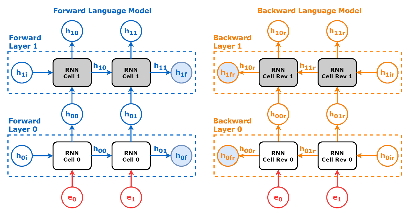
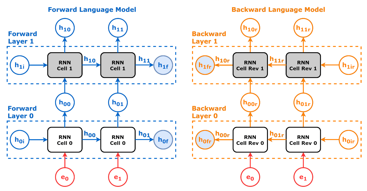
ELMo generates word embeddings by incorporating context from the entire sentence, allowing the representation of words to change based on their usage.
It uses a bidirectional LSTM architecture, processing text both forwards and backwards, and stacks multiple layers for deeper contextual understanding.
ELMo embeddings are derived from all layers of the network, where lower layers capture syntax and higher layers capture semantic features.
The design focuses on pre-trained deep language models that are task-agnostic, making ELMo adaptable to various downstream applications by integrating into existing pipelines.
BERT (Bidirectional Encoder Representations from Transformers)
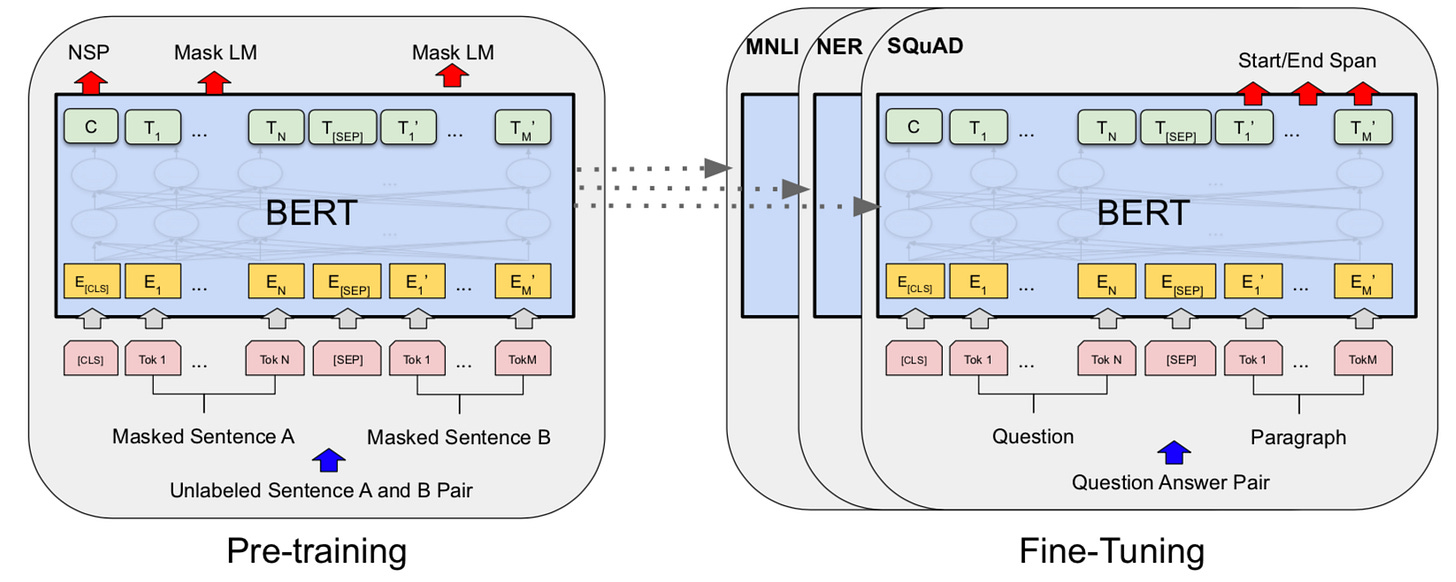
BERT is based on the transformer architecture and leverages self-attention mechanisms to model the full context of words within a sentence.
Unlike traditional unidirectional models, BERT uses bidirectional attention, enabling it to consider both preceding and succeeding words simultaneously.
Its design includes multiple layers of transformers, with each layer refining representations using multi-headed self-attention and feedforward neural networks.
BERT’s flexibility is highlighted by its ability to handle sentence-pair tasks, such as question answering and textual entailment, in addition to single-sentence tasks.
Pre-Training Approaches for Contextual Embeddings
ELMo Pre-Training
ELMo is pre-trained on a large corpus using a language modeling objective. Specifically, it employs two separate objectives: forward prediction (next word prediction) and backward prediction (previous word prediction).
This dual-directional training allows ELMo to capture both past and future context in its embeddings.
Example: Generating ELMo Embeddings
from allennlp.commands.elmo import ElmoEmbedder
# Initialize ELMo Embedder
elmo = ElmoEmbedder()
# Input sentence
sentence = ["This", "is", "an", "example", "sentence", "."]
# Generate embeddings
embeddings = elmo.embed_sentence(sentence)
# Each word has three vectors (from different layers)
for i, word_embedding in enumerate(embeddings):
    print(f"Word {sentence[i]}: {word_embedding.shape}")  # Example: (3, 1024)
BERT Pre-Training
BERT introduces two novel pre-training objectives:
Masked Language Modeling (MLM): Randomly masks words in a sentence and trains the model to predict the masked words using context from both directions.
Next Sentence Prediction (NSP): Trains the model to predict whether a given sentence follows another in a sequence, improving its ability to handle tasks involving sentence pairs.
These objectives allow BERT to develop a nuanced understanding of both sentence structure and inter-sentence relationships.
Generating BERT Embeddings
from transformers import BertTokenizer, BertModel
import torch
# Load pre-trained BERT tokenizer and model
tokenizer = BertTokenizer.from_pretrained('bert-base-uncased')
model = BertModel.from_pretrained('bert-base-uncased')
# Input text
text = "This is an example sentence."
# Tokenize input text
inputs = tokenizer(text, return_tensors="pt", padding=True, truncation=True)
# Generate embeddings
with torch.no_grad():
    outputs = model(**inputs)
# Extract last hidden states
last_hidden_states = outputs.last_hidden_state
print("Shape of embeddings:", last_hidden_states.shape)
# Example: torch.Size([1, 7, 768]) -> (batch_size, sequence_length, hidden_size)
Fine-Tuning Contextual Embeddings
Fine-Tuning ELMo
ELMo embeddings are typically used as additional input features to downstream models.
By freezing or slightly adjusting the weights of the pre-trained ELMo model, its embeddings can be fine-tuned to specific tasks like named entity recognition (NER), sentiment analysis, or question answering.
Fine-Tuning BERT
BERT is fine-tuned by adding a task-specific head (e.g., classification, regression, or sequence generation layers) on top of the pre-trained transformer layers.
During fine-tuning, the entire model is updated to optimize task-specific objectives, making BERT highly adaptable to diverse NLP applications.
Techniques like gradient clipping and learning rate warm-up are often employed to stabilize training and prevent catastrophic forgetting of pre-trained knowledge.
from transformers import BertForSequenceClassification, AdamW
from transformers import Trainer, TrainingArguments
# Load pre-trained BERT model for classification
model = BertForSequenceClassification.from_pretrained('bert-base-uncased', num_labels=2)
# Define tokenizer and data
tokenizer = BertTokenizer.from_pretrained('bert-base-uncased')
# Example dataset
texts = ["I love this!", "This is awful."]
labels = [1, 0]  # Positive = 1, Negative = 0
# Tokenize data
encodings = tokenizer(texts, truncation=True, padding=True, max_length=128, return_tensors="pt")
# Prepare dataset
class Dataset(torch.utils.data.Dataset):
    def __init__(self, encodings, labels):
        self.encodings = encodings
        self.labels = labels
    def __len__(self):
        return len(self.labels)
    def __getitem__(self, idx):
        item = {key: torch.tensor(val[idx]) for key, val in self.encodings.items()}
        item['labels'] = torch.tensor(self.labels[idx])
        return item
dataset = Dataset(encodings, labels)
# Training arguments
training_args = TrainingArguments(
    output_dir='./results',
    num_train_epochs=3,
    per_device_train_batch_size=8,
    evaluation_strategy="epoch",
    save_steps=10_000,
    save_total_limit=2,
    logging_dir='./logs',
)
# Define trainer
trainer = Trainer(
    model=model,
    args=training_args,
    train_dataset=dataset,
)
# Train model
trainer.train()
Chapter 2 provided a comprehensive foundation for understanding text representation techniques and contextual embeddings, which are essential for modern NLP systems. We began with classical approaches like Bag-of-Words and TF-IDF, progressing to advanced distributed representations such as Word2Vec, GloVe, and FastText. These methods emphasized capturing semantic meaning and efficient representation of text.
The chapter further explored embeddings like ELMo and BERT, which introduced the power of contextualized word representations. By discussing their architectures, pre-training strategies, and fine-tuning methodologies, we established a strong understanding of how these embeddings capture rich linguistic context and contribute to various NLP applications.
As the landscape of text representation has evolved, so too has the need for models capable of leveraging these representations to generate coherent and contextually relevant outputs. This brings us to the next chapter, where we focus on the progression from traditional statistical language models to modern neural network-based approaches.
If you have any inquiries, feel free to reach out via message or email.
Connect with me on Linkedin
Find me on Github
Visit my technical channel on Youtube
No posts
Comments
Nothing yet. Say the first thing.
Sign in to join the conversation.