Simulating Graneau's Copper Bars Experiment

This post elaborates on my commentary:

The swapping of components refers to if they are different components not the same and so that would not apply in this case but was merely an example of the exhibition of voltage difference because in this example the two components are exactly the same so swapping them would not change anything but I still hold to voltage difference is the cause of the situation but does not fully explain the results what you add to it is the magnetohydrodynamics and thermal shock further explains the consequences of voltage difference driving the two rods apart but the initiation and the motivating force is voltage difference and here’s the explanation the voltage gradient through the simple loop circuit puts a mathematical average of 0 volts in between the two rods as a consequence of one rod being the same magnitude of voltage as the other but of opposite polarity so one rod is positive while the other is negative and zero stands between them now zero is merely a mathematical average it is not the reality the reality is perturbations of various imbalances over time that causes the froth of the universe so to speak the baseline noise of the universe that is considered to be quantum in nature but it really doesn’t matter whether we call it quantum or femto or Pico the scale doesn’t matter what matters is that it’s small and that it varies over time but that variation over time creates the thermal shock necessary and the pressure the thermal pressure necessary to push the two rods apart using standard magnetohydrodynamic principles of the liquid mercury but what put that froth that boiling froth there in the first place is something called a virtual ground in which it might be zero volts on average over time but at any particular moment in Time it is nearly zero but not exactly and not consistently zero because it changes with a zero overall average and that’s what creates the Dynamics but it’s nearly zero so it’s the froth of the universe so to speak and that creates turbulence in no uncertain terms because it’s at the dividing line between the positive rod and the negative rod because it’s nearly zero it’s considered a virtual ground even though it’s not an official ground and that points out another sidebar that’s not related to your post but is related to my study of ground electrical grounds are sometimes an additional contribution to a circuit’s energy because they’re zero but they’re only zero as a mathematical average over time in reality potentially they are the source of the froth of the universe in other words a source of turbulence that can be harnessed to initiate oscillations across them and if the wave mechanic is designed to accumulate rather than dissipate then that oscillation will build rather than not exist at all or diminish but the fact that the turbulence is potentially there is what this experiment by Ampere [Graneau]1 is exhibiting and that turbulence is a potential source of energy that is used to push the rods apart which in a sense is over unity you know the appearance of over unity but it’s not really over unity over time because it mathematically averages out and thus supports conservation of energy but at any moment in time conservation of energy is not applicable and that creates the turbulence that’s when conservation of energy does not apply to any particular moment in time when the turbulence is arising even though it’s microscopic or quantum or whatever size of scale it is it’s there really small and it changes over time and that drives the turbulence and so that shows that a ground rod is the point of turbulence (very small) that could be harnessed to become something larger but that’s a sidebar the main theme is that the fact that the rods are sitting in Mercury doesn’t require a whole lot of turbulence to push them apart but it does show apparent over unity even though it’s chaotic it also shows chaos and that’s a prime feature of nonlinear Dynamics and the appearance of other unity from one moment compared to the next moment because it’s overall over time there is no over unity but from one moment compared to the next there is so it’s really a question of discreet analysis that produces the appearance of over unity rather than the overall big picture which does not.

That description deserves a graphic which can segue into a series of similar simulations — similar, in the sense that a substantial source of D/C voltage is not always required to produce magnetohydrodynamic turbulence between two copper rods sitting immersed in a mercury bath although I include that elevated voltage version in the third simulation.

This turbulence — in the gap between the rods — is sufficient to push them apart due to the thermal shock which results from the elevated temperatures which this turbulence will provoke according to Dr. Paul Wilhelm’s analysis of Graneau’s experiment (if I understand and quote Dr. Wilhelm’s analysis, correctly).

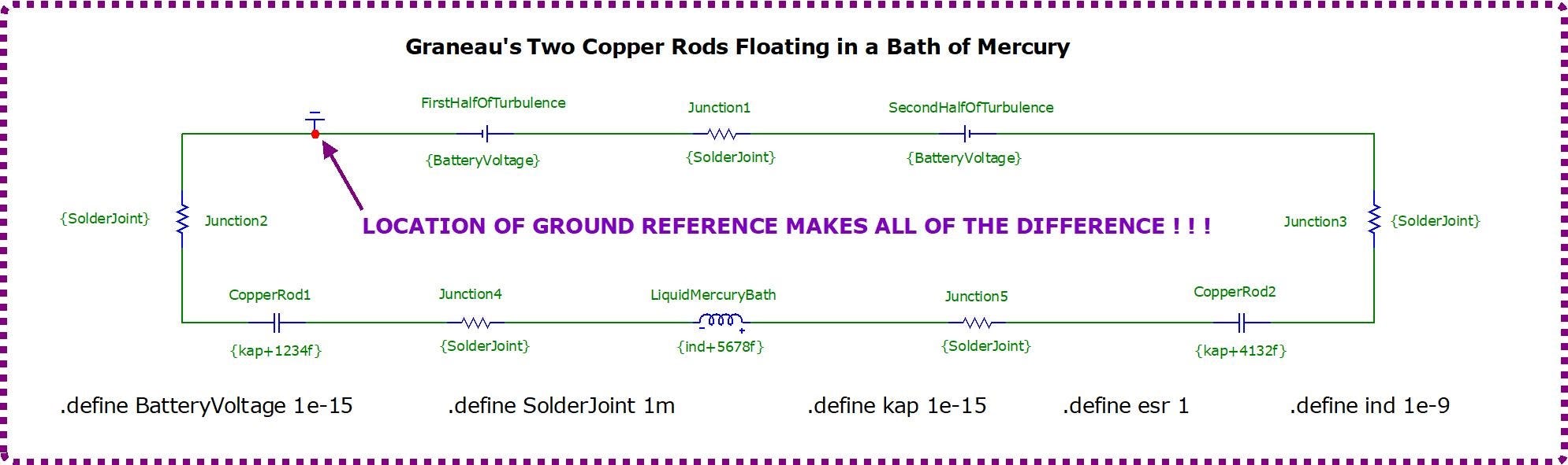
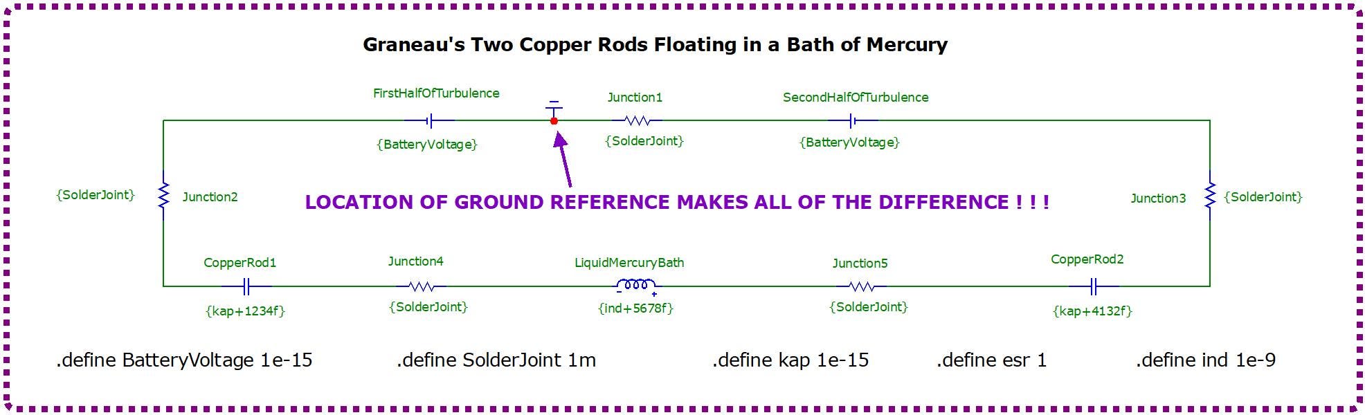
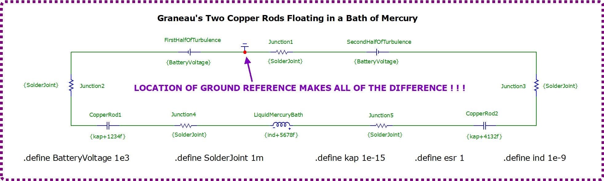
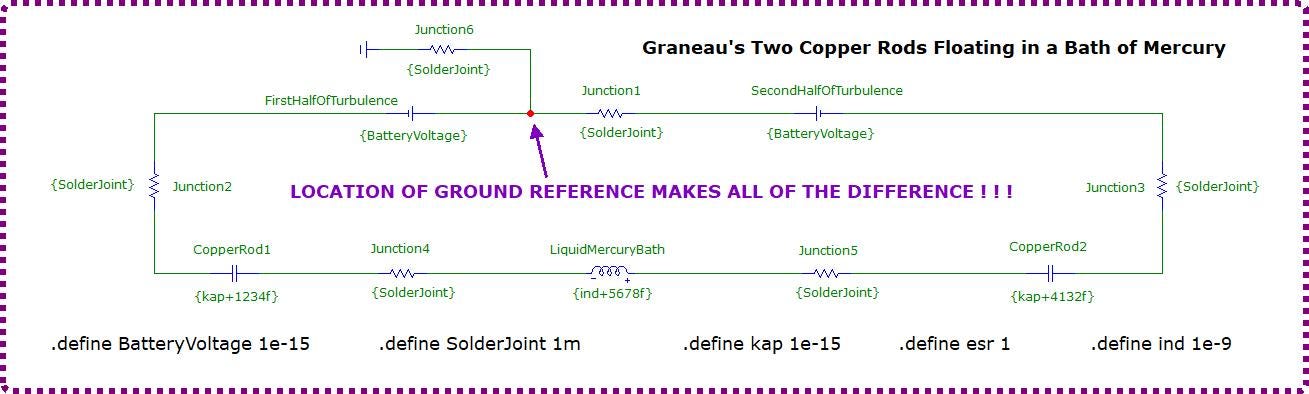
I represent this turbulence — and the gap between the pair of copper rods which encompasses this turbulence — by opposing two batteries of opposite polarity but of equivalent voltages. I use two versions of battery voltage: 1e-15V for simulations #1 and #2 versus 1e+3V for simulation #3. So, these two virtual (ie, non-existent) batteries sit in between the two copper rods in the miniscule gap adjoining their contact surfaces prior to their separation upon the application of a D/C voltage (resulting in the flow of current) through their copper length and through their mercury bath.

I represent the mercury with an inductance and place this in between a pair of capacitors which represent each copper rod.

So, a question could arise as to which does the pair of batteries represent versus what does the inductor represent since we have two candidates: the gap between the rods versus the other gap on the opposite side of this simple looped circuit where Graneau’s battery (voltage source) was located? »»»

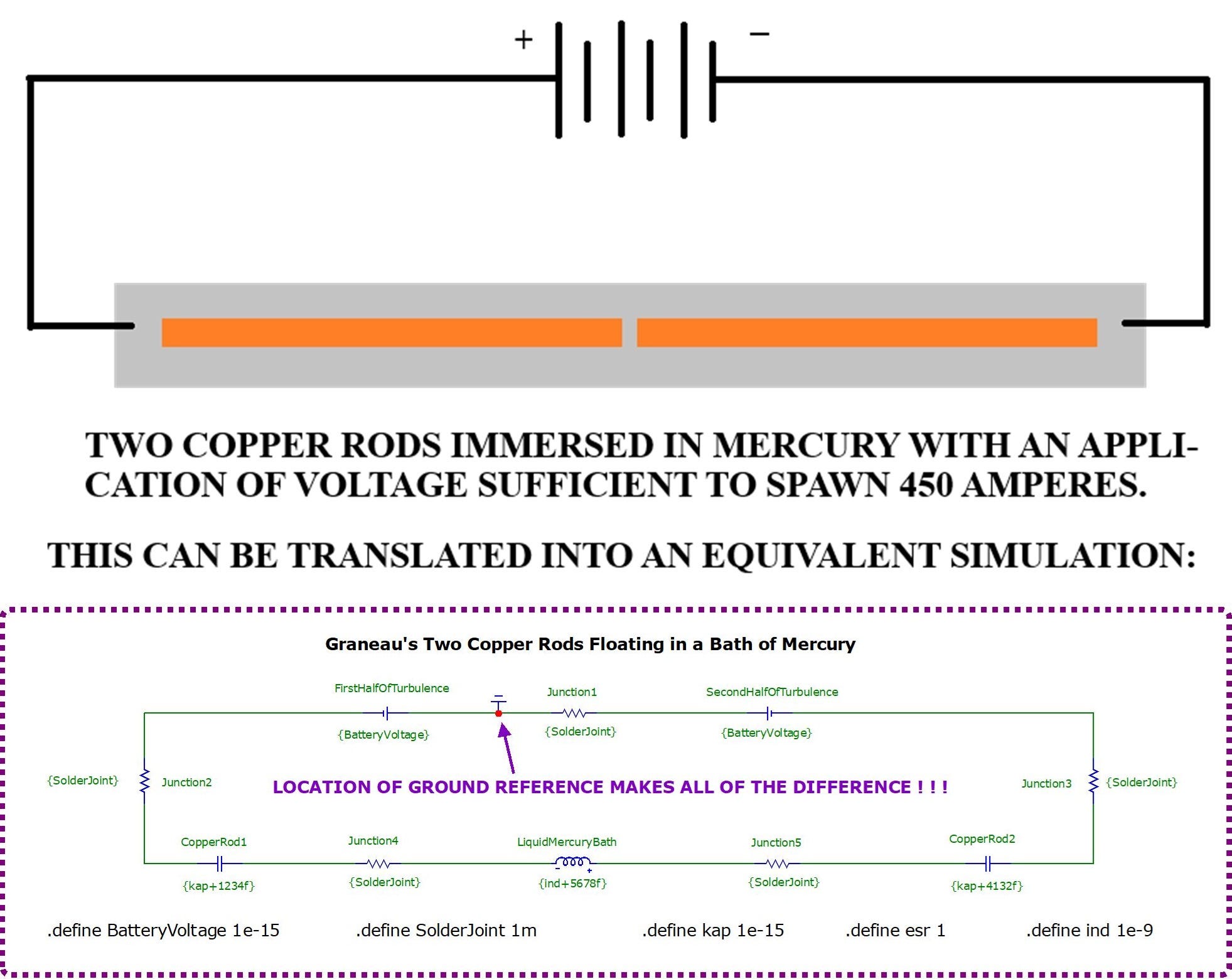
My guess is that the opposing pair of batteries represents the turbulence between the copper rods (since the voltage of these two batteries are in opposition to each other) while the inductor represents Graneau’s voltage source. That sounds awkward (according to conventional reasoning) but makes more sense than making an opposing pair of batteries represent a single battery.

My precedence for labeling the inductor as a source is that it is going to become a voltage source when a pair of batteries oppose each other’s voltages. The inductor will become a generator since it will also violate (or, transcend if you prefer) the Law of Induction by Michael Faraday by becoming a source of negative watts based on whatever voltage is applied to this inductor’s two terminals but without the necessity of moving this inductor through a magnetic field.

Instead, all that is needed is a turbulence of voltage upsetting uniformity (spawning chaos: the mother of nonlinear dynamics).

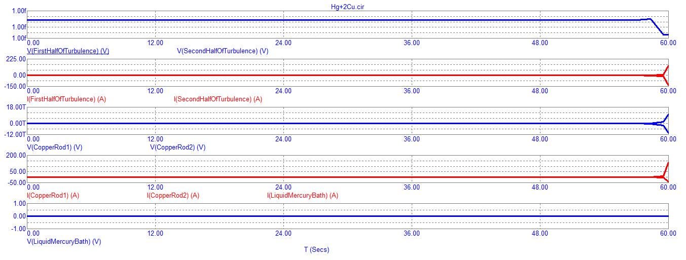
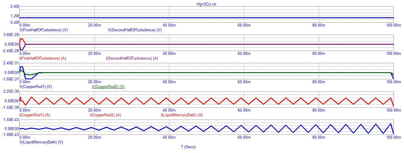
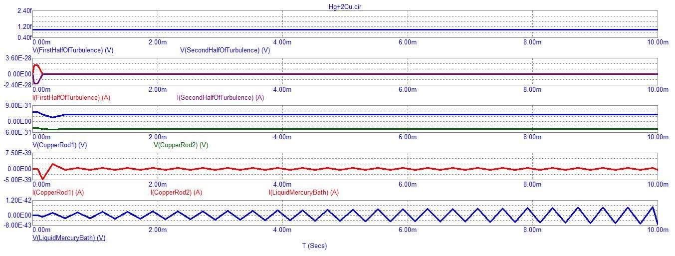
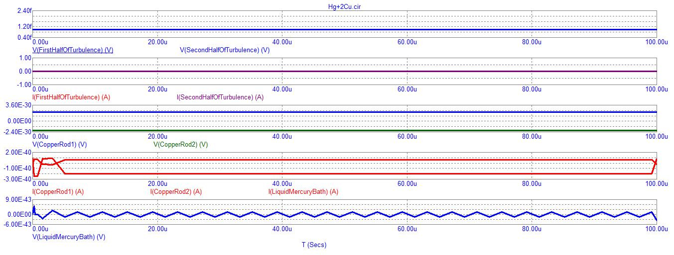
So, three versions of this simulation are undertaken. The first version (circuit filename: “Hg+2Cu.cir”) has its ground reference off to one side (to the left of the pair of opposing batteries) and each battery is rated at 1e-15V, namely one femto volt:

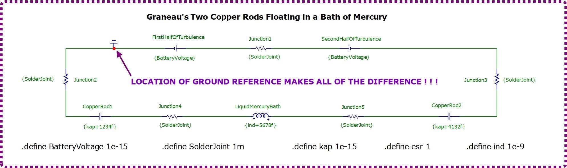
By the way, the inductor’s internal series resistance has been set to a unit value equal to its inductance to approximate a wire gauge of 25 AWG. So, an inductance of one nano Henry, at a wire gauge of 25 AWG, will possess an approximate internal series resistance of one nano Ohm according to my derivation from the measurements which Dr. Roger Hastings applied to the Joseph Newman table model version of the Newman device and referencing standard wire gauge charts and tables. This analysis of the Newman circuit was published in chapter six of Newman’s book.

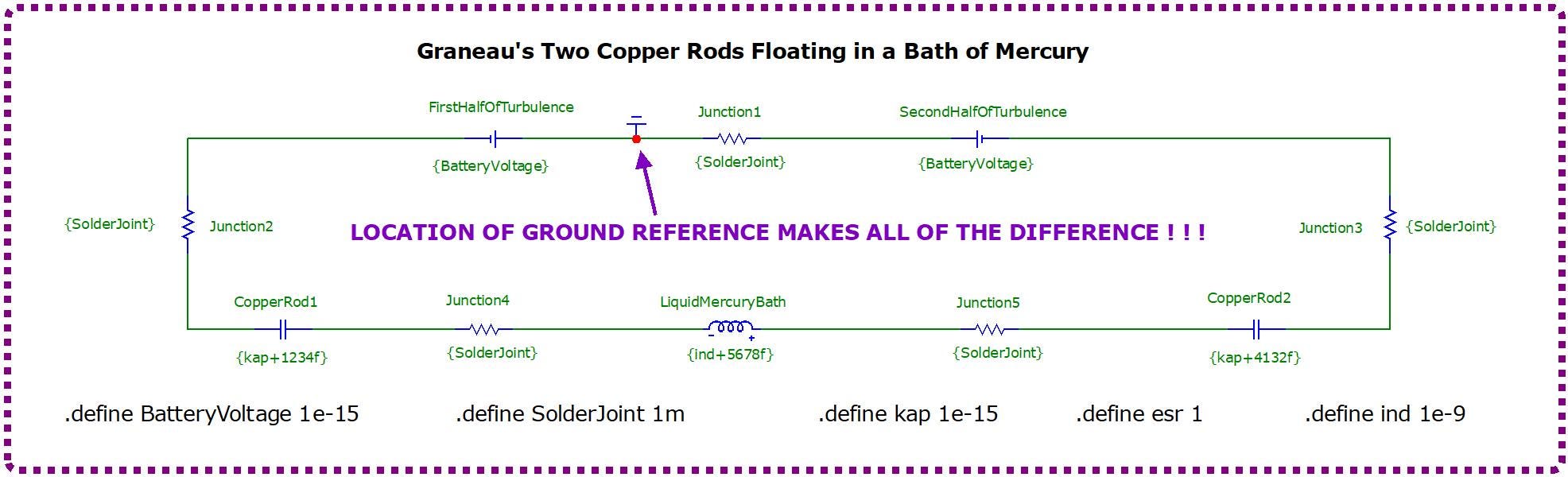
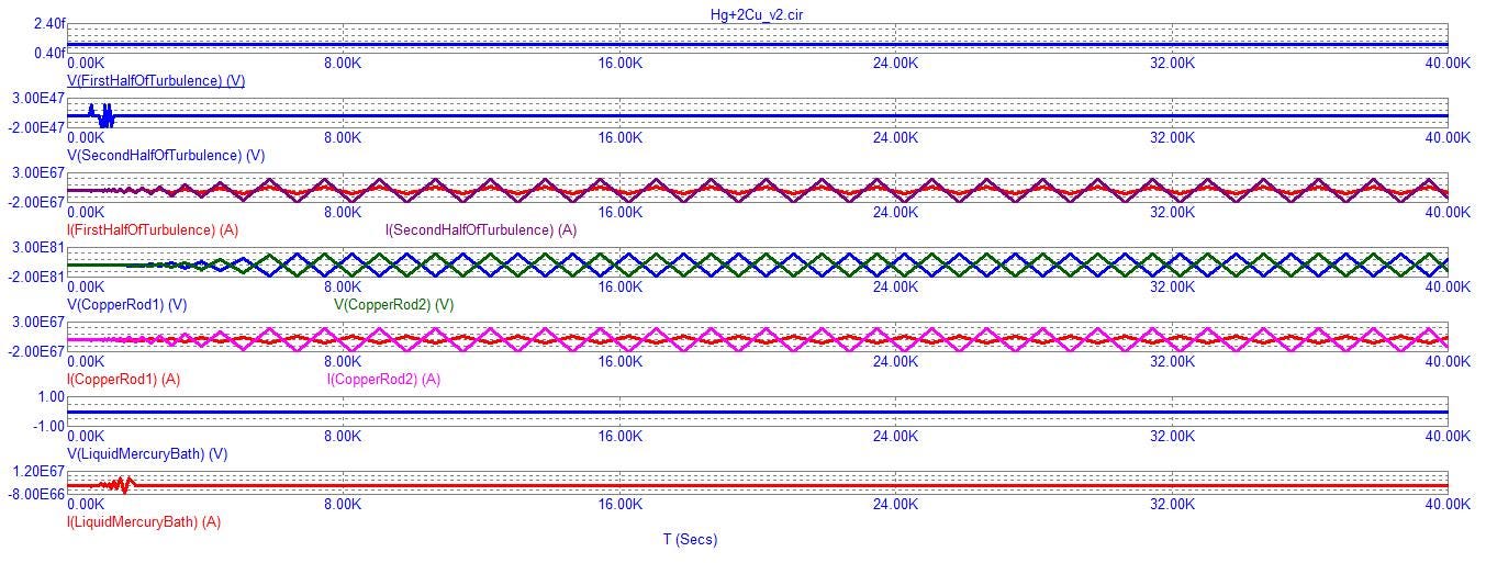
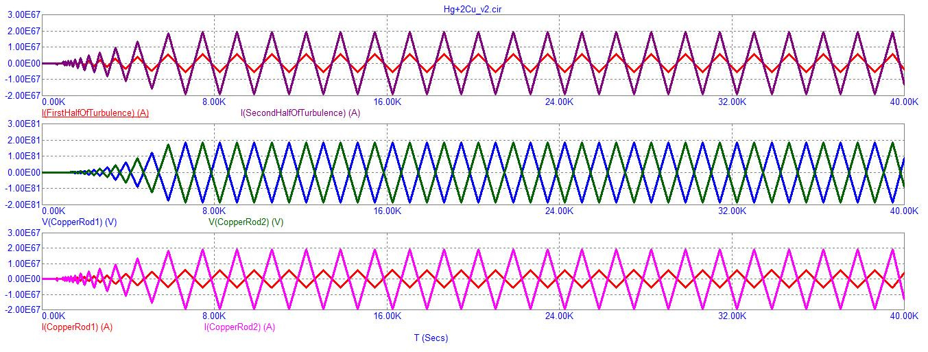
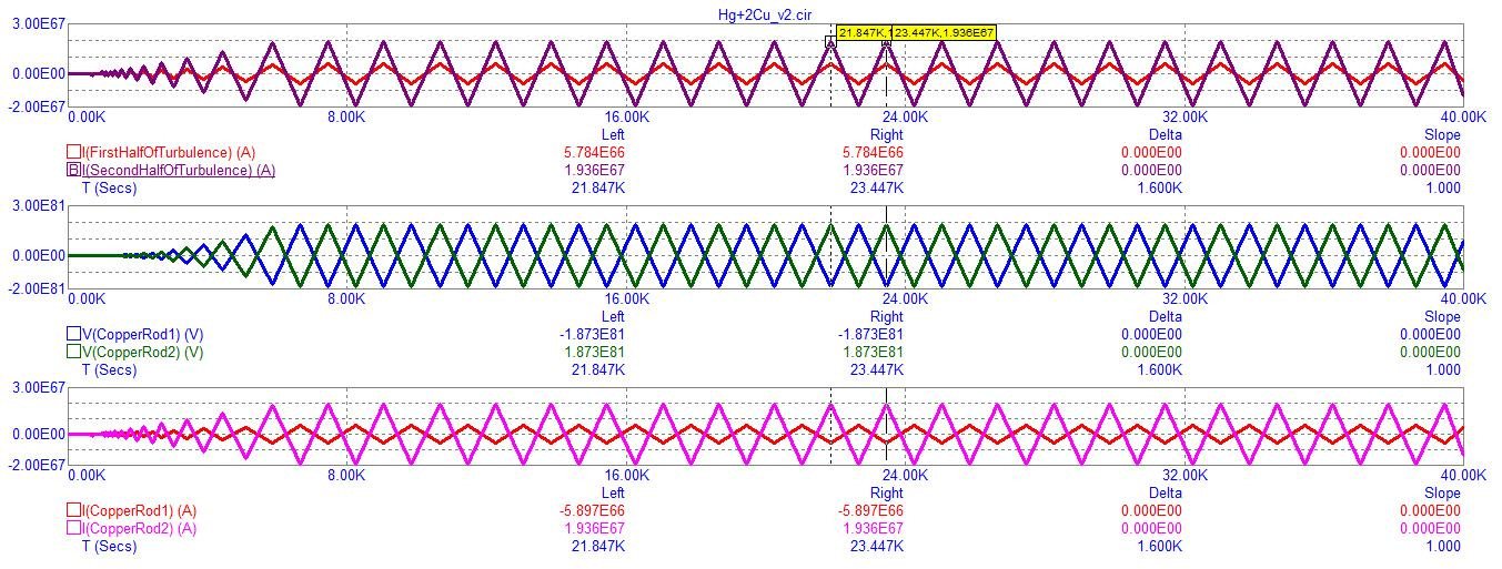
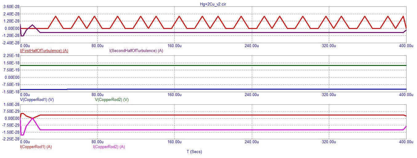
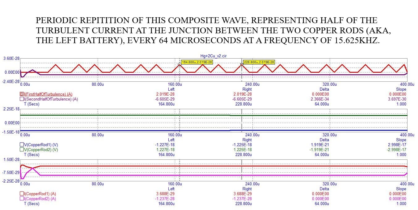
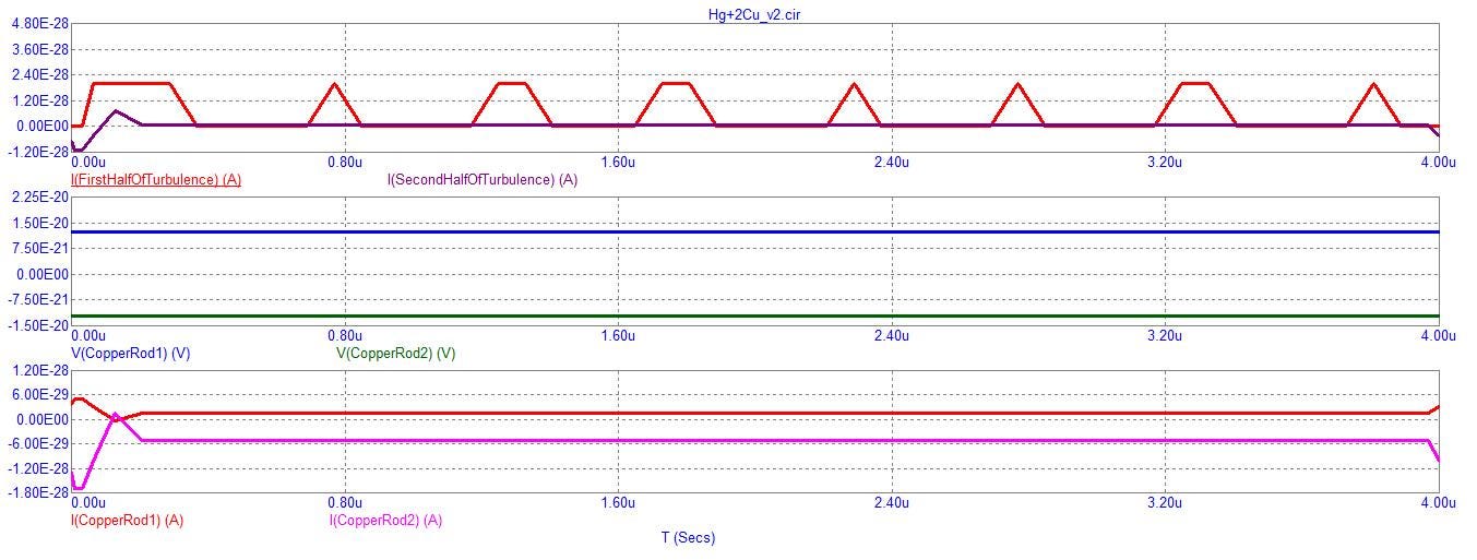
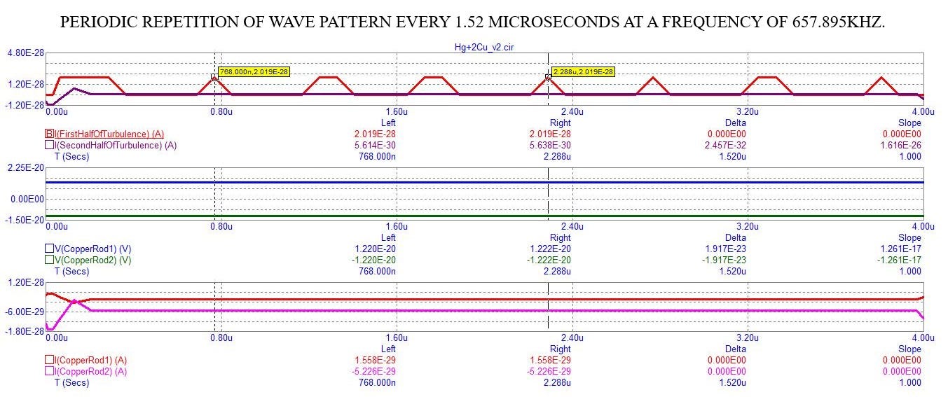
The second version (circuit filename: “Hg+2Cu_v2.cir”) has its ground reference shifted closer to the center of the turbulence — occurring between the opposing voltages of the pair of batteries at the top of these schematics — while using the same low voltage of the previous version #1 of 1e-15V for each battery:

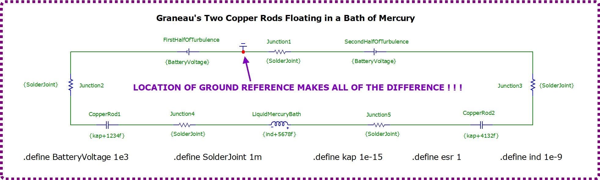
The third version uses the same location for its ground reference as does version #2, above, but elevates the voltage of each battery to 1e+3V, namely one kilovolt:

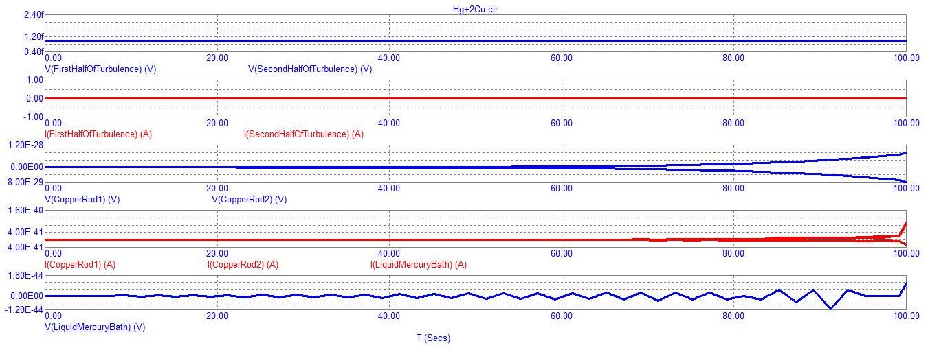
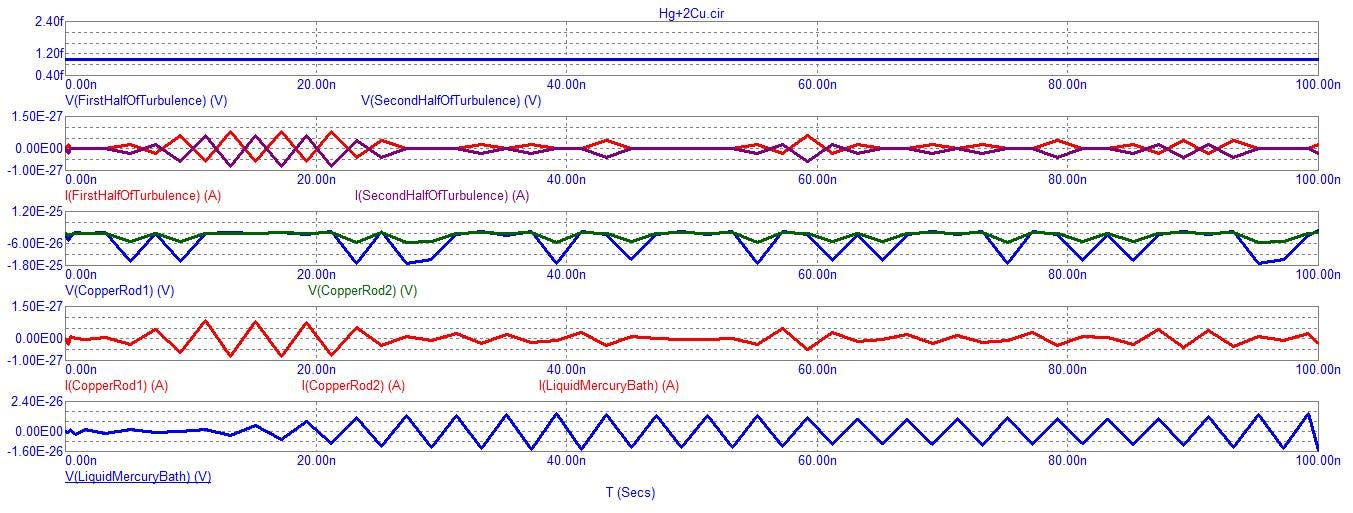
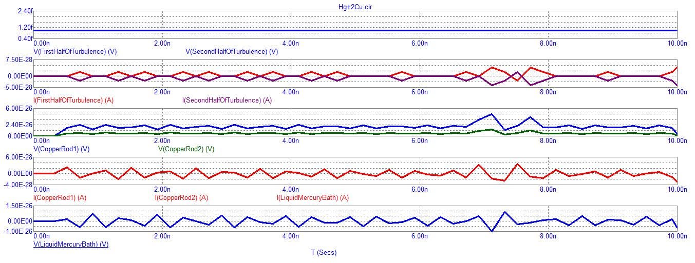
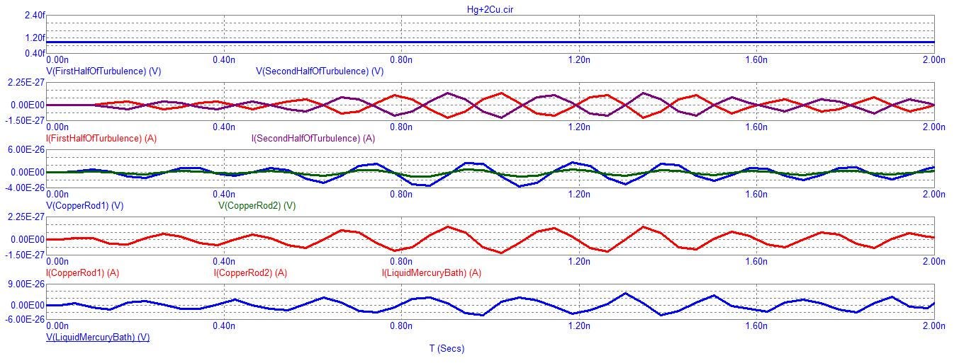
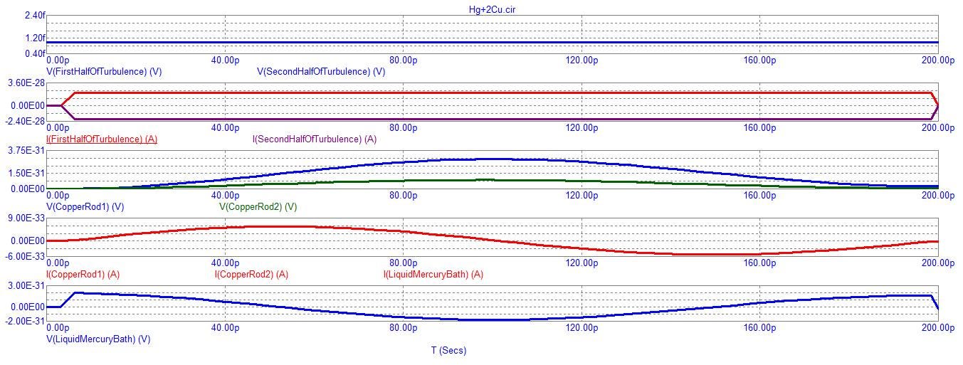
The outcomes are very interesting due to their graphical and numerical variations among diverse runtimes. Yet, there are two distinct themes which keep repeating themselves: either the outcome will flatline due to the opposing voltages from each of the pair of batteries cancelling each other out, or a turbulence will result. The simulator, obviously, can’t make up its mind or else the same waveforms would manifest regardless of various runtimes.

This dualistic outcome epitomizes conventional wisdom versus Dr. Wilhelm’s findings: that a flatline should result under the auspices of conventional expectations. But a turbulence should result if we include all of the elements of Maxwell’s theory as described by Dr. Wilhelm in many of his recent posts. These discrepancies occur due to averaging, over time, which upholds Conservation of Energy versus moment to moment which does not due to microscopic imbalances which always occur in reality. Only within the realm of statistical averaging does Conservation hold true. And yet, this average is loosely equivalent to our observations at the level of what we can see with our own eyes. But at the level of microscopic vision, the Froth of the Universe becomes apparent.

This “froth”, or perturbations, can be magnified under specific conditions which just about all of my “free energy” experimental simulations have sought to embody.

So, in theory, I know these disturbances exist and can be accessed if a successful translation of any of my simulations is possible into a real-world build.

This is why I can’t give up my pursuit of simulating anomalous circuitry outcomes since the theory of electrodynamics encompasses every contrast in theory that a person could pose — especially now that we have access to computational accuracy with the advent of 64-bit registers. My recent tally of a free energy circuit, which could be mistaken to be overunity, agrees with the Conservation of Energy yet raises a serious question about the extent of “sources” in conventional physics. These conventions may be restricted to “politically correct” sources, alone, ignoring a few sources which sit outside of “acceptable standards of expectation” as reported to us by way of Eric Dollard.

Well, enough with the expository writing. On with the show! …

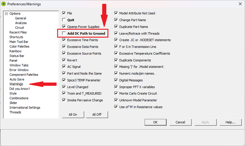
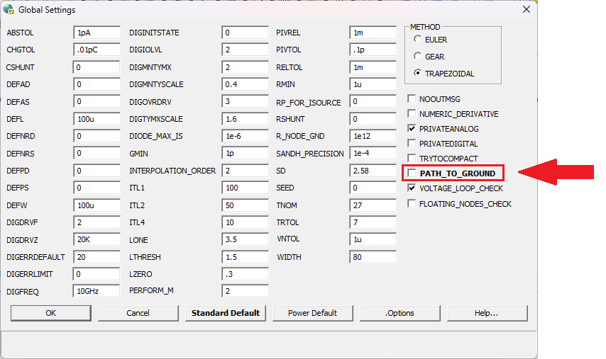
The following three screenshots are of settings within Micro-Cap’s “Preferences” and “Global” which must be “unchecked” so as to avoid warnings which have no useful bearing upon these experiments and merely get in the way (by preventing the simulator from accepting these simulations during runtime):

Here is schematic #1:

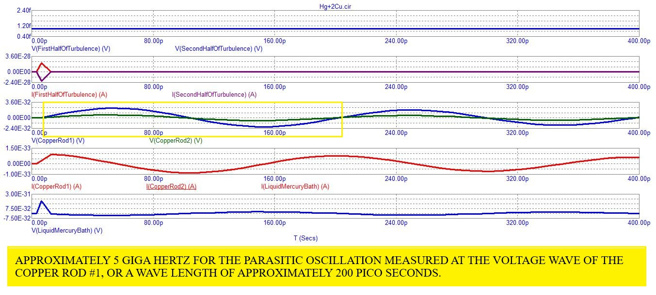
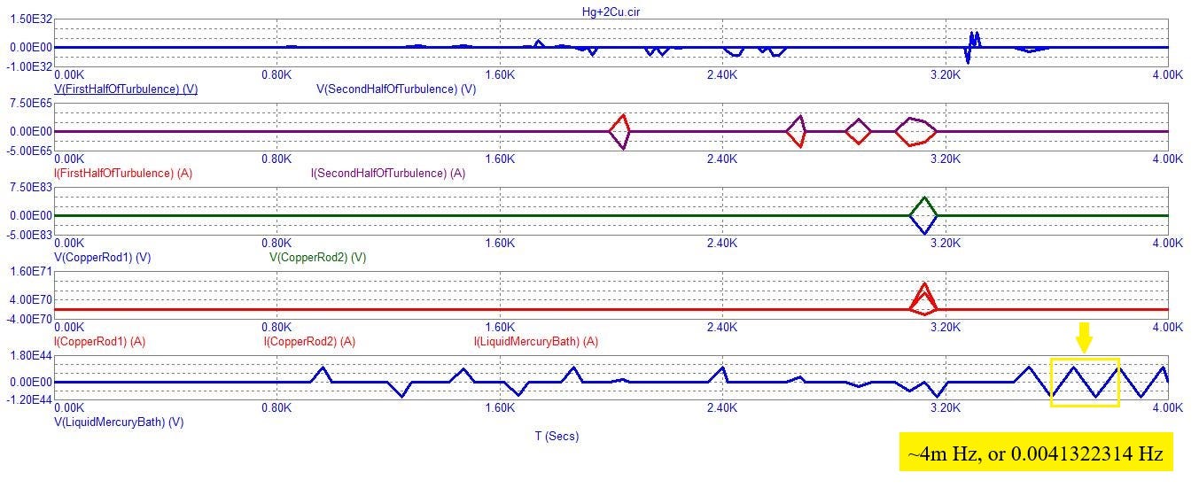
Here is the second schematic:

And, finally, here is schematic #3:

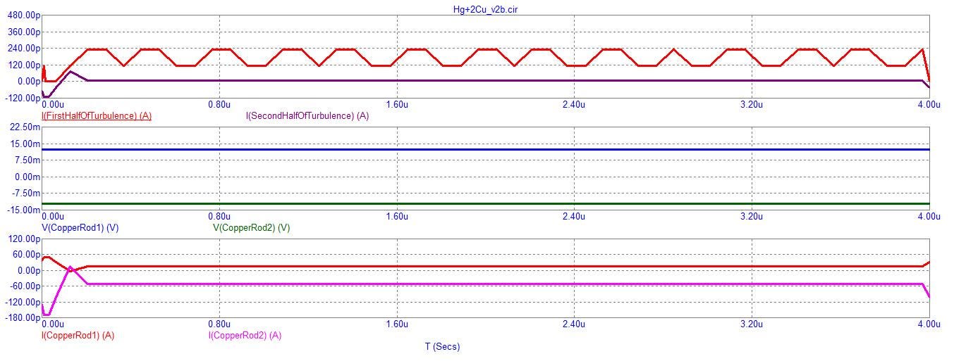
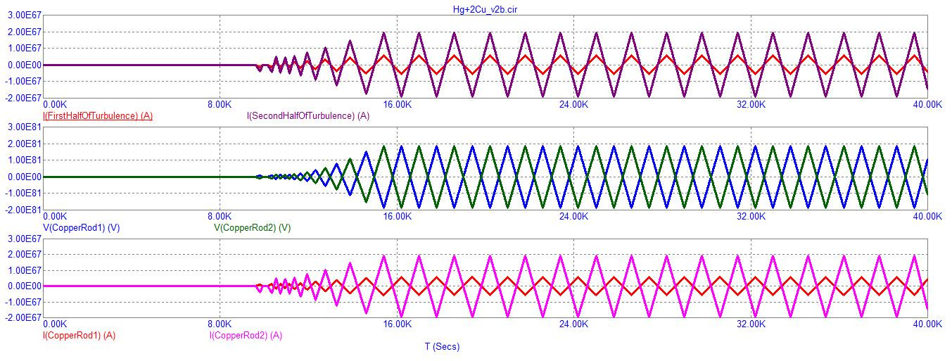
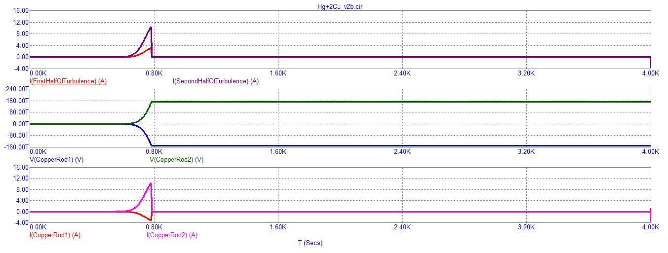
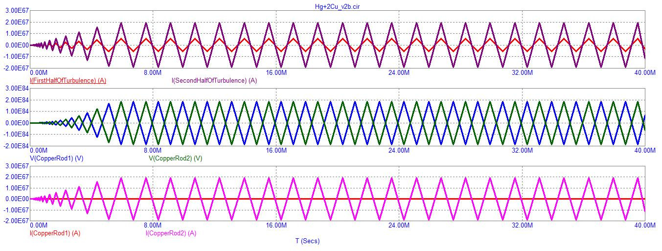
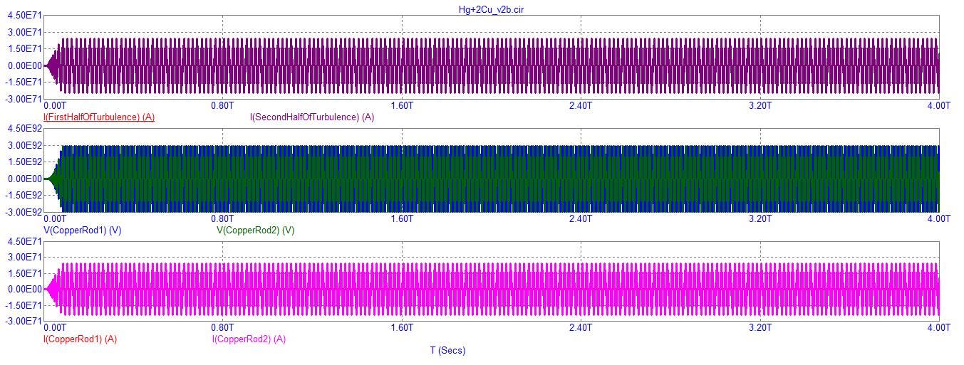
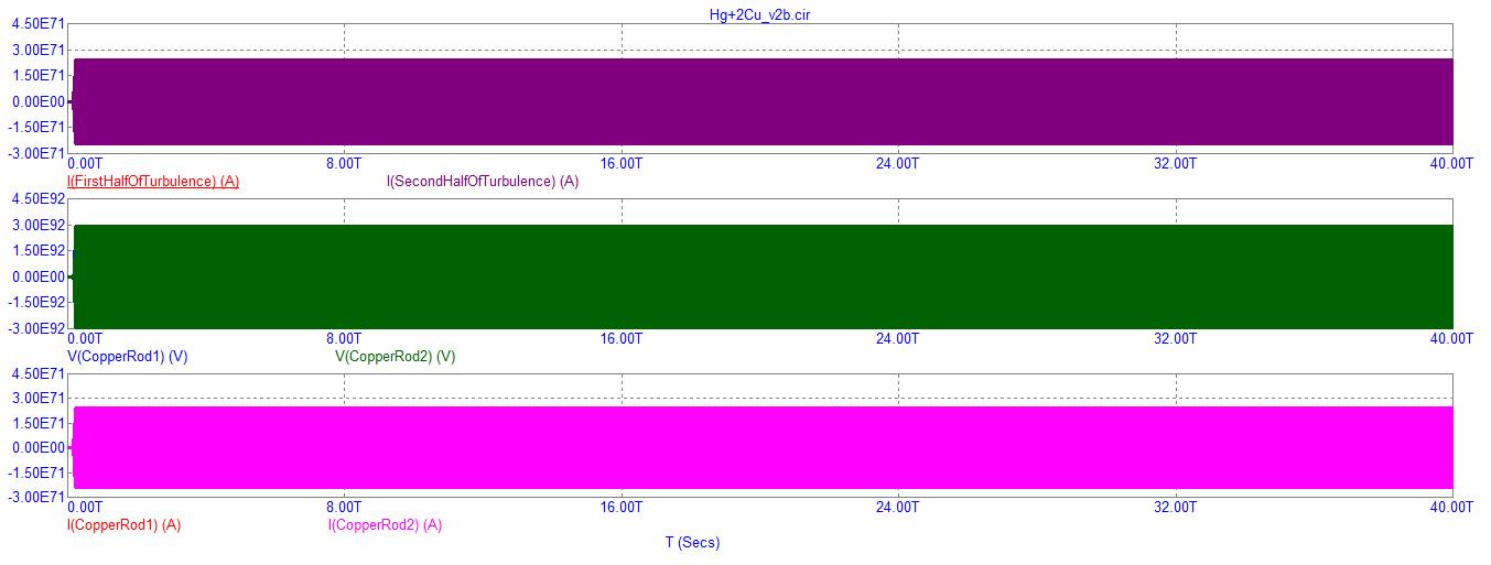
Most of the time, the only variation among all of these different outputs is a variation of runtime: “For how long did I run each circuit simulation within each of these three general contexts of minor circuit variations?”

Download this experiment from my website or from my Google Docs account.

In retrospect, I did not do these simulations sufficient justice since I left out a wattage tally of every single component. So, let’s give it a try and see what happens …

Schematic for the following “tally” experiment:

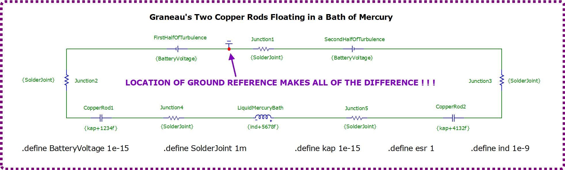
Not any different than the second schematic from before, eh?

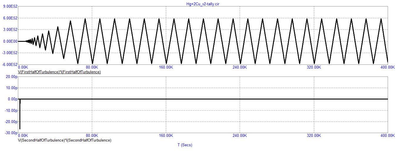
Turbulence of the pair of the femto-volt batteries as measured by their raw wattage waveforms:

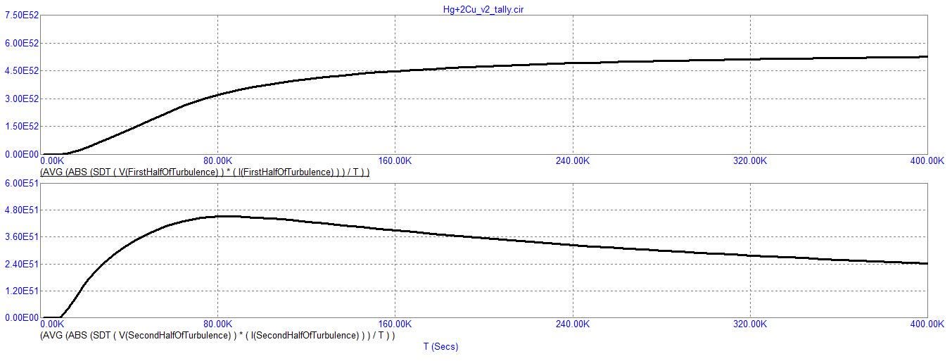
Turbulence of the pair of the femto-volt batteries as measured by their SDT averaged, wattage waveforms:

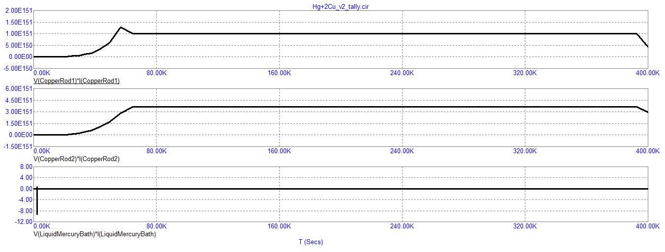
Inductance and capacitances of the entire system traced in their raw waveforms:

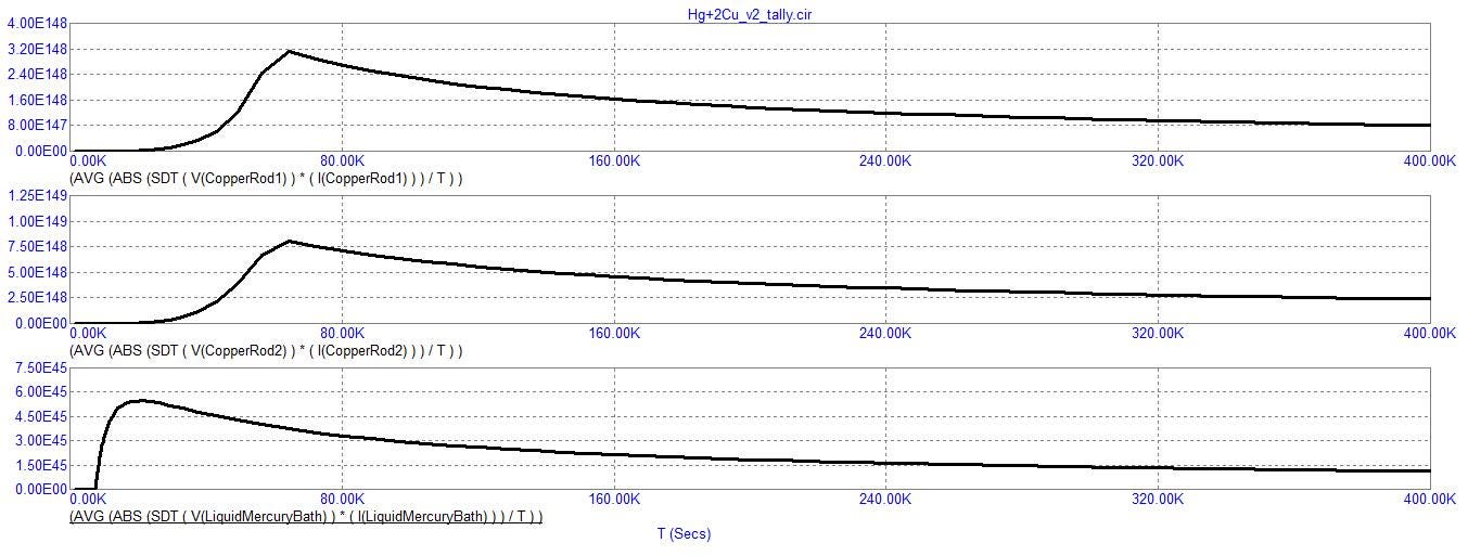
Inductance and capacitances of the entire system traced in their averaged SDT waveforms:

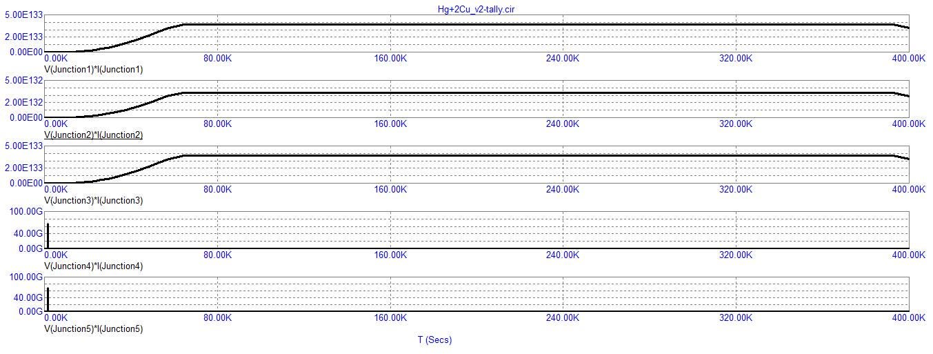
The five junctions among the virtual components of this “system” in their raw waveform tracings:

The five junctions among the virtual components of this “system” in their SDT averaged waveform tracings:

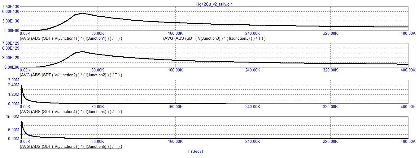
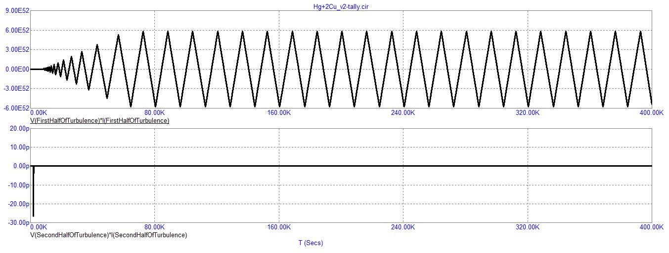
By the looks of these tracings of the SDT averages of the wattages of all of the components of this simulation, I’d say that an initial surge occurs which quickly or slowly dissipates in all of the components except in one-half (the first half) of the turbulence which slowly rises to a plateau and will probably remain there.

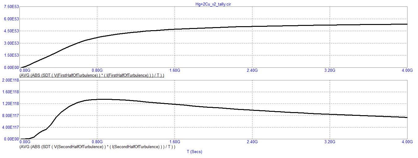
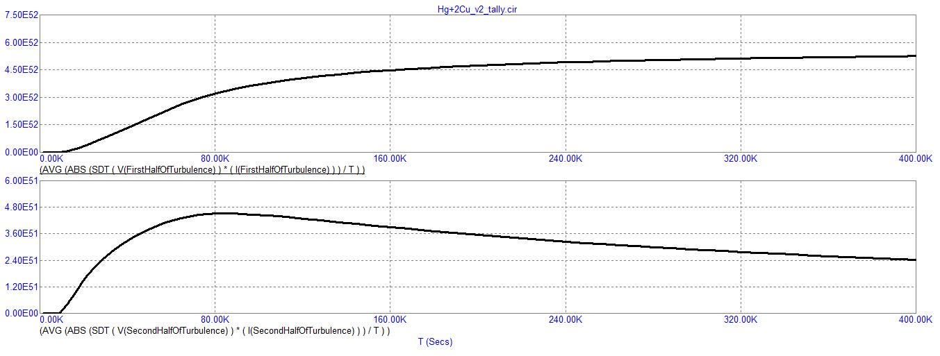
Since the turbulence is fictional, it could be deduced (or hypothesized) that the overall turbulence is partly subdued (due to the low value of the “secondhalfofturbulence” which merely spikes in the beginning) and partly very active (due to the plateau of elevated spiked waveforms of the “firsthalfofturbulence”).

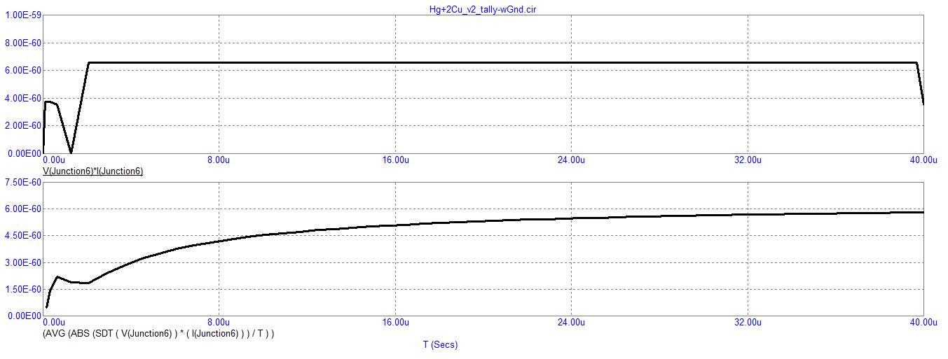
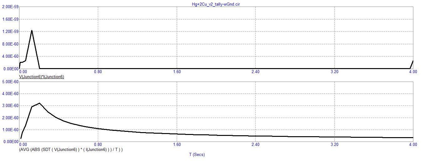
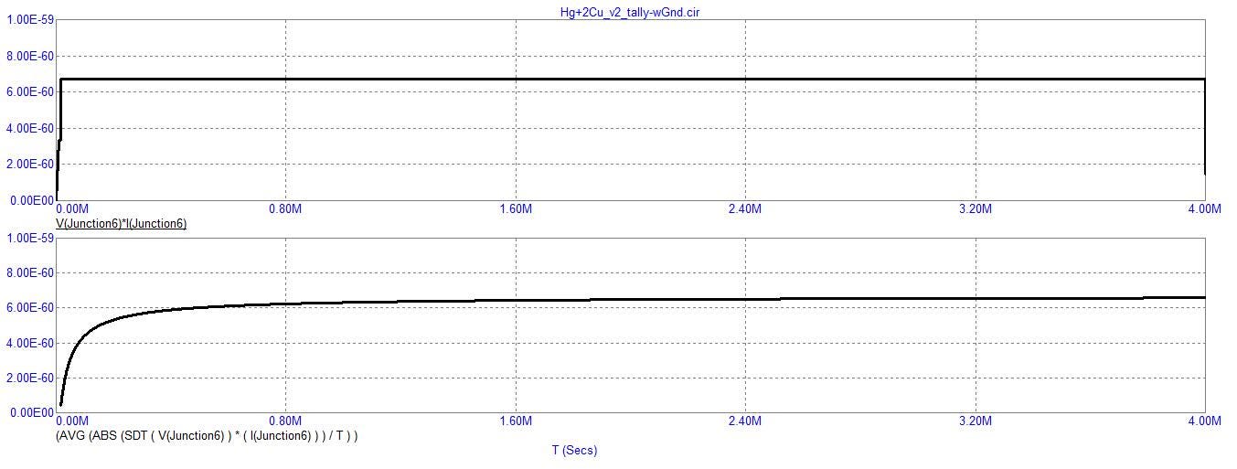
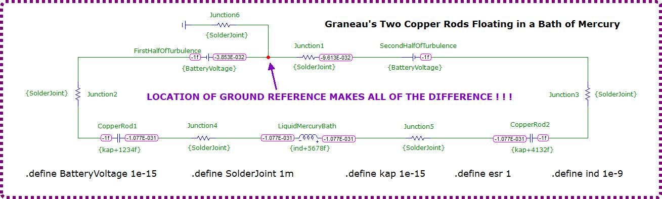
I forgot to include the ground as part of my analysis since it wasn’t in Graneau’s original experiment. But it cannot be overlooked since the simulator demands I put at least one ground into the schematic. So, what happens if it’s analyzed (labeled: “Junction6”, below, in the upper left-center of the screenshot)?

Output at 40 microseconds:

Output at 4 seconds:

Output at 4 kiloseconds:

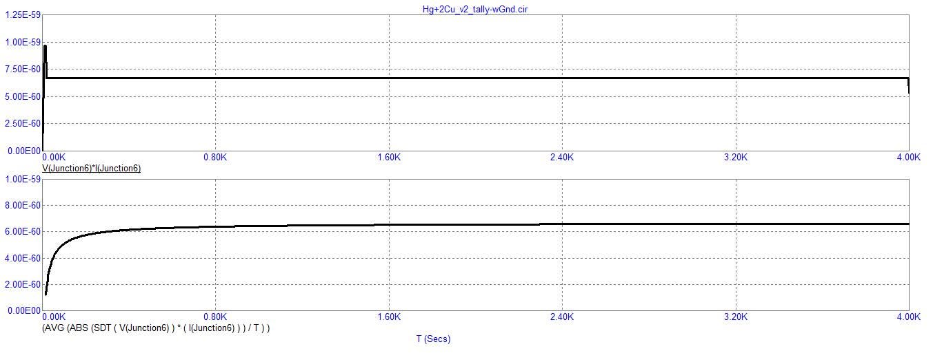
Output at 4 Mega seconds:

Nodal Voltages at 4 Mega seconds:

Currents at 4 Mega seconds:

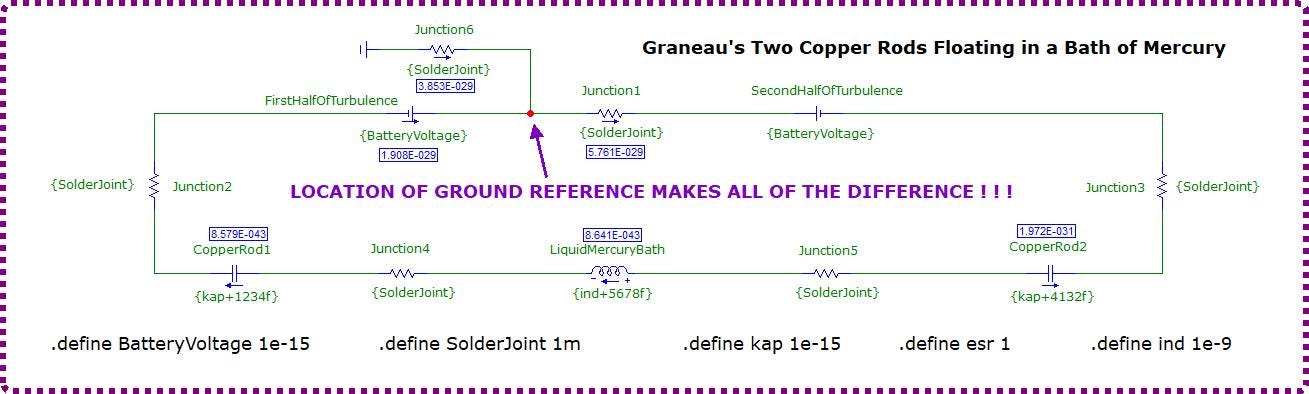
Powers at 4 Mega seconds:

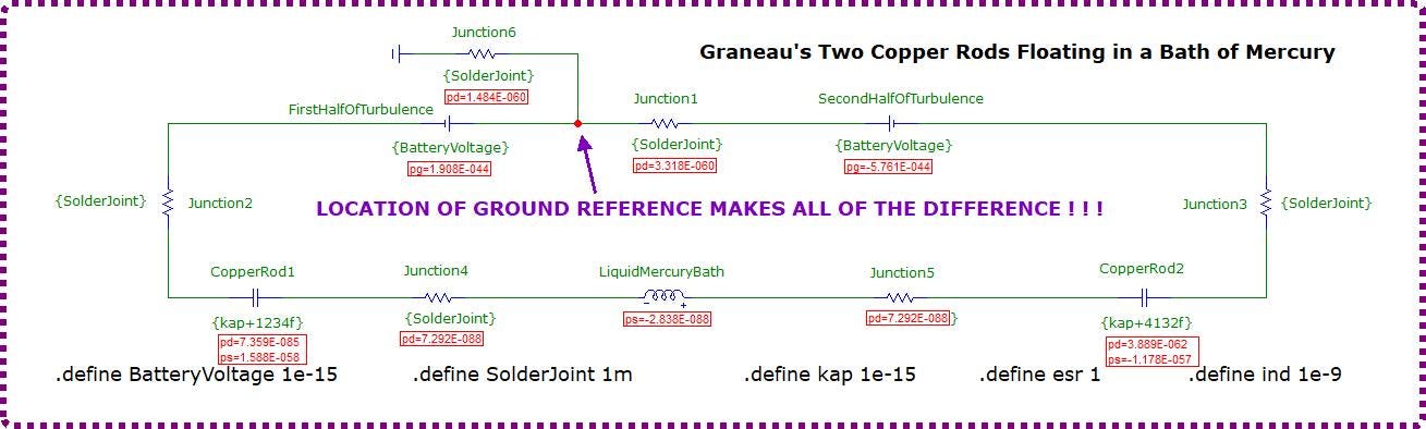
But the looks of this latest screenshot of the powers distributed across this circuit, we see that negative watts is located at the “LiquidMercuryBath” inductor in the format of reactive storage, and at the “CopperRod2” capacitor (also) in the form of reactive storage. Also worth noting is that positive watts (indicating the recharging of a battery rather than its expenditure) is occurring at the D/C battery labeled: “FirstHalfOfTurbulence”.

These are all small figures which don’t surprise me since a little turbulence (imbalance) can go a long way in achieving incredible results if the energy accumulates rather than dissipates.

My conclusion is that, without this additional resistor (labeled: “Junction6”), the simulator blows up one of its pair of batteries. But since nothing undergoing explosive reaction actually becomes destroyed when undergoing simulation (since this is virtual reality), the explosive battery supplies lots of power to the rest of the circuit and the rest of the circuit quickly loses its ability to entertain any power while quickly dissipating it.

Is this free energy? No, it’s one of a pair of batteries which act as if it is shorted out through a superconductor operating at room temperature — which is no small feat in itself!

So, something anomalous is happening.