My Third Successful Free Energy Circuit Prevents a Runaway Condition in which Conservation of Energy is Upheld without Errors since the Amplitudes are Regulated

The purpose behind this dialogue with AI is for it to help me regulate a circuit. I already know how to turn its surge ‘ON’ versus ‘OFF’. So, all I need is a dynamic protocol to regulate the outcome in real-time.

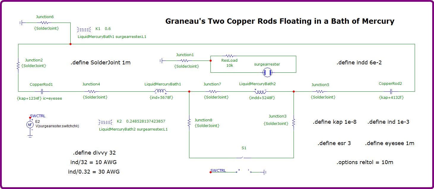
I do this by using a switch, labeled: ‘S1’, which is fed a control signal from a behavioral voltage source, ‘E2’, based on whether the surge arrester has come ‘ON’. This ‘ON’ condition is discovered by measuring the voltage of node #10 of the surge arrester’s macro. This node is also labeled with the convenient name of: ‘Switchchk’. So, testing for voltage (of this node) is easy: tell the behavioral voltage source to measure the voltage of this node by using the test statement of: ‘V(surgearrester.switchchk)’ and feed this as a control signal, labeled: ‘SWCTRL’, to the switch to tell the switch to turn itself ‘OFF’ and, thus, ‘OPEN’ the switch to kill the surge which spawned this state of plasma within the surge arrester.

This plasma status, within the surge arrester, is what is dangerous for this particular circuit configuration risking a runaway self-destructive condition. In other free energy circuit configurations, this hazard may manifest in a different format requiring a different set of protocols to manage that situation.

The ‘OFF’ condition is induced by using a combined inductance of 0.061 Henrys. That’s 61 millihenries. It’s ‘ON’ condition is maintained with a combined inductance of 0.001 Henrys, or 1 millihenry. This elevated inductance of 61 millihenries smothers the instability of free energy production within this circuit.

Low levels of reactance parameters tend to induce free energy more often than not.

“Instability” is what electrical engineers are brainwashed (ie, taught) on how to interpret a free energy condition for that is the “nature of the beast” of runaway reactance.

It is reactance that will generate free energy if this reactance is of the type which can clone itself via ‘non-inductive reactance’ and ‘inductive acceptance’:

This is a very explosive condition which is also a safety hazard if not managed.

This inductive ‘OFF’ combination is brought about by adding up the two inductances of ‘LiquidMercuryBath1’ and ‘LiquidMercuryBath2’. The ‘ON’ condition is brought about by excluding ‘LiquidMercuryBath2’ from any active engagement by cutting off its electrical connection by use of a switch which opens up and disconnects its throughput from the circuit.

The ‘OFF’ condition is when switch ‘S1’ closes due to a signal it receives letting it know that the surge arrester has come ‘ON’. The Konzen circuit behaved differently in as much as its surge arrester promoted its free energy production. But in this instance, the surge arrester’s participation gets in the way of this circuit’s safe operation (aka, free from self-destructive tendencies). So, whereas the surge arrester in this circuit helps induce a surge when it is both ‘ON’ or when it is ‘OFF’, the surge condition must be shut ‘OFF’ whenever the surge arrester is ‘ON’ to prevent a dangerous runaway escalation of amplitude.

So, the switch pulses — automatically; on its own without any explicit micromanagement from me, but from implicit micromanagement from the circuit sensing when the surge arrester comes ‘ON’ and closing the switch to engage the extra inductance which will turn the circuit’s surge condition ‘OFF’.

By the way, I give a few hints as to how to calculate American Wire Gauge (AWG) by specifying that a wire gauge of 10 AWG can be achieved by dividing a coil’s inductance by 32, etc. This relation I deduced from reviewing wire gauge charts plus the measurements which Dr. Hastings rendered of the tabletop model of the Joseph Newman device which the good doctor shared with us in chapter six of the Newman text.

Here is the finished circuit:

Don’t be alarmed at the elevated ‘reltol’ parameter above its usual default of 1m.

On the schematic, above, this ‘reltol’ parameter is defined with the statement in the lower right-hand corner of the schematic: “.options reltol = 10m”.

This instance of the modification of ‘reltol’ does not alter the behavior of this circuit at all. Its elevation merely makes it easier for the simulator to render the outputs in support of the Conservation of Energy. But the surge-like behavior of this circuit remains unaffected by the alteration of ‘reltol’.

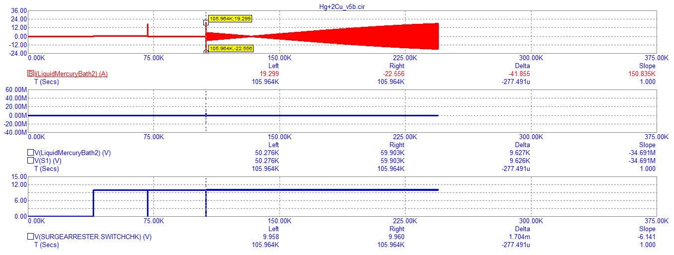
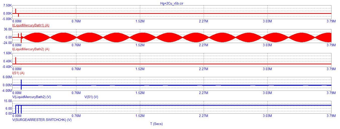
This circuit is very well-regulated. See how the current is very stable once it reaches its plateau at around 106 kiloseconds (specifically 105,964 seconds):

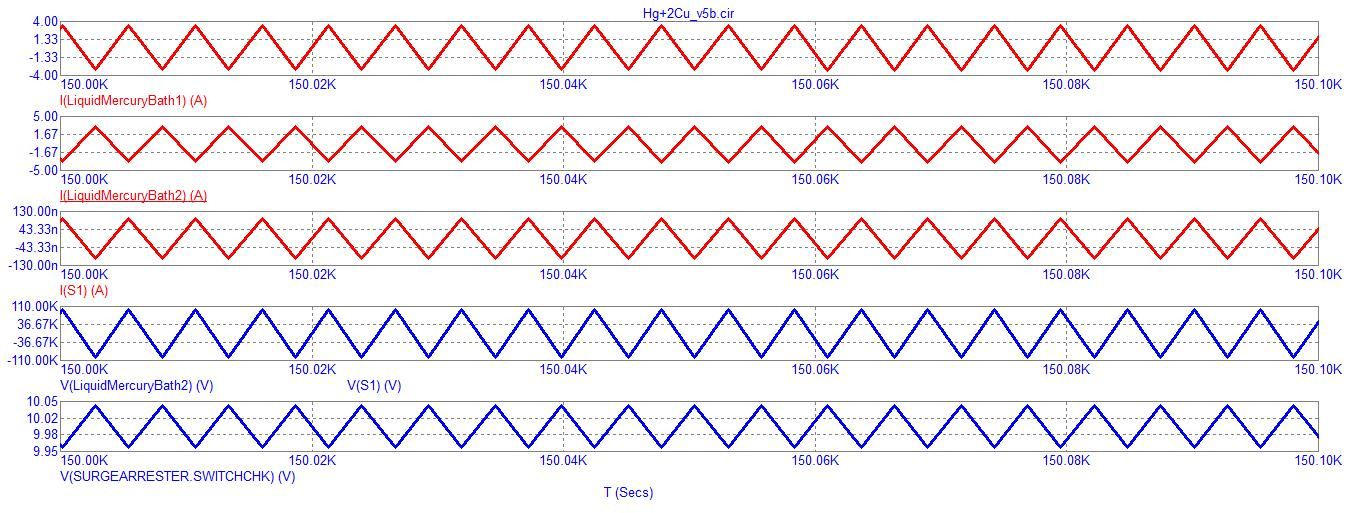
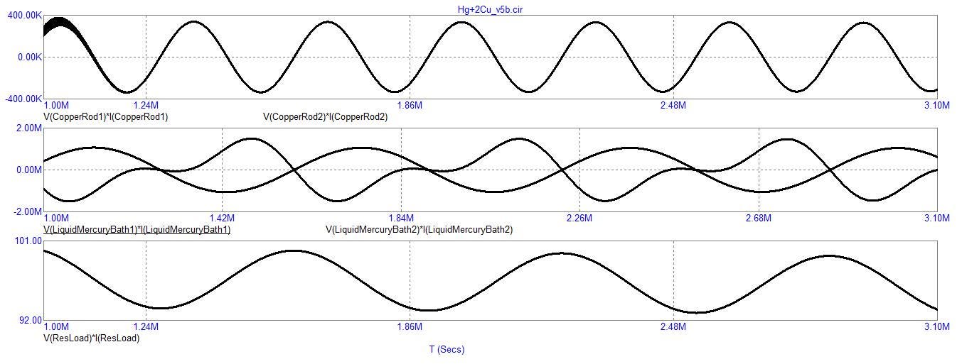
Here’s a closeup view of some of the currents and some of the voltages:

Funny that a bunch of triangular current and voltage waveforms can spawn sine wave wattages: [huh?]

Maybe those triangle waves (up-above) are not triangle waves after all? Maybe they’re merely the real-number values of the plots of the peaks and troughs of each wave and the simulator connects those sparse tracings misleading us to conclude that they are triangle waves when, in fact, they may be the ONLY real-numbered data points of what is — for the most part — a tracing of an imaginary wave existing most of the time within the realm of imaginary numbers: ie, the square roots of negative numbers?

It makes sense since the multiplication of an imaginary voltage times an imaginary current results in negative watts. And negative watts is the passive sign conventional definition of the production of energy which may be analogous or equivalent to Eric Dollard’s use of the term: “inductive acceptance”.1

Notice how the wave in the topmost graph is refining itself in that a smaller amplitude wave, which is riding piggy-back on top of the main wave, is reducing its amplitude and, thus, shrinking the oscillatory bandwidth of this piggy-back wave in the far left-hand side of the topmost graph.

This parasitic amplitude had surged, in the beginning, but is -now- damping itself down since regulated switchings have taken over contributing the main ingredient of this circuit’s overall behavior.

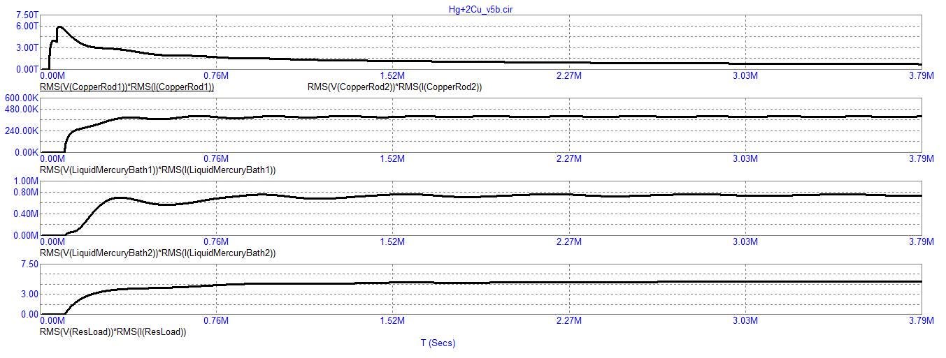
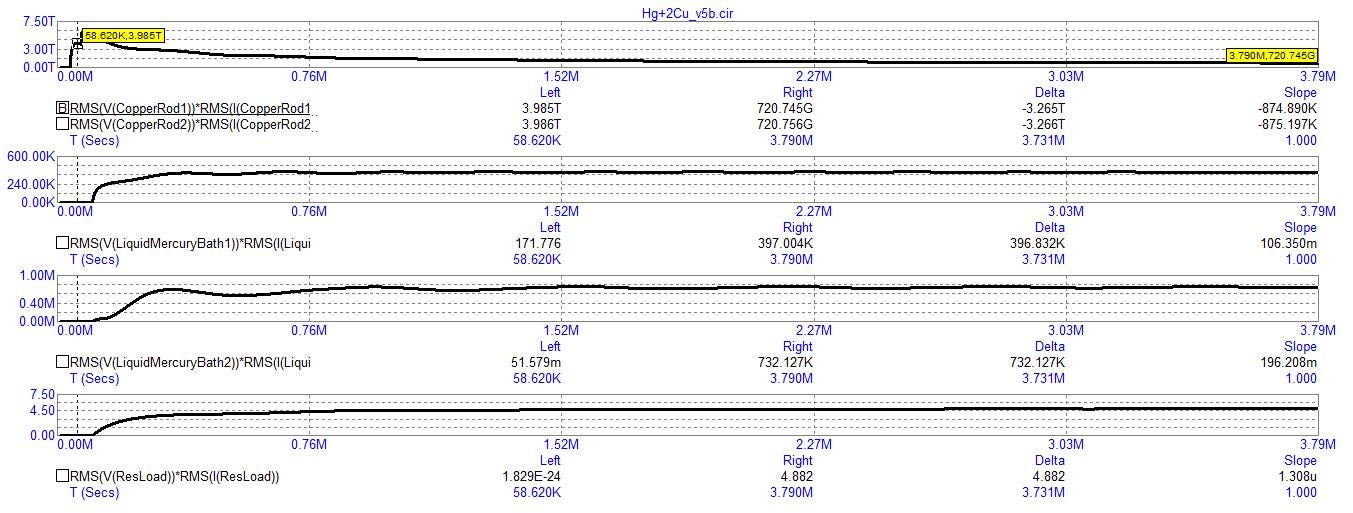
Thus, due to the prevalence of sine waves (in evidence up-above), I can use RMS to calculate the average wattages:

Download this experiment from my website or from my Google Docs account.

[The prior discussion with ChatGPT was lost. But we managed to recover the gist of it.]

please continue our previous discussion

Absolutely. We were working on your Micro-Cap coupled-inductor circuit, specifically the subcircuit where you were trying to make the magnetic coupling change when an inductor’s inductance doubles.

The key correction from our last exchange was:

• L3 must be included.

• You do not want the middle-row configuration I had inferred.

• You want the third row.

• In that desired configuration:

  • K₁ = 0.6

  • K₂ = 0.24853

• The reason for introducing the second coupling coefficient is that when the relevant inductance changes, the mutual coupling must change with it, rather than leaving the coupling relationships fixed.

So we should pick up from that third-row configuration, not redesign the circuit around the middle row.

If you paste/upload the latest Micro-Cap .cir/subcircuit again, I can continue directly from the exact equations/netlist and show you the precise Micro-Cap syntax needed to implement K₁ = 0.6 and K₂ = 0.24853 with L3 included, including what Micro-Cap objected to in your attempted implementation.

I have the uploaded sparkgap(2).mac. This is the Micro-Cap display/settings file for the Spark Gap macro, rather than the actual macro definition itself.

I checked it specifically for the Switchchk behavior we were discussing. This file does not contain the circuit equations or the G1 behavioral current source; it contains things such as analysis-window settings, waveform display settings, and simulation options.

So it doesn’t yet give us the piece we need to modify the inductance/coupling.

The relevant Spark Gap macro information from our previous work was:

• Switchchk is the control node.

• G1 uses V(SWITCH,PIN2) * V(SWITCHCHK) as its controlling expression.

• Switchchk is approximately 10 nV in the off state and 10 V in the on state.

• You want an inductor to change from 1 mH → 2 mH when Switchchk = 10 V, and return to 1 mH when Switchchk = 10 nV.

• L3 must remain part of the magnetic-coupling system.

• Your desired third-row coupling arrangement is:

  • K₁ = 0.6

  • K₂ = 0.24853

The important issue is that the .mac file you just uploaded isn’t the file containing the L and K statements.

If you upload the actual Spark Gap macro circuit file (or the .cir file containing the three inductors and K statements), I can work directly from it and determine exactly how to implement the two coupling states without running into Micro-Cap’s prohibition on a variable inductance in a K statement.

Yes — this is the actual circuit file, and now I can see exactly where we left off.

There is an important point in this version that changes how I would approach the solution.

Your schematic currently has only one physical inductor:

LiquidMercuryBath
inductance = {ind+5678f}

and your definition is:

.define ind {1e-3+indie}
.define indie {if(V(surgearrester.switchchk)>=10,1e-3,0)}

So the inductor is presently:

• 1 mH when switchchk < 10 V

• 2 mH when switchchk >= 10 V

That part of your approach is actually doing what you intended.

You also have one K element:

K1
INDUCTORS = LiquidMercuryBath surgearrester.L1
COUPLING = 0.6

So K1 = 0.6 is already present.

There is no L2 or L3 in this particular .cir file.

That explains the Micro-Cap objection we were dealing with earlier: you can’t make the coupling statement behave as though the inductance change itself automatically creates a new coupling coefficient. The K element is a relationship between specific inductors, and Micro-Cap doesn’t permit the approach of simply putting a variable inductance expression into the K relationship in the way we were attempting.

And this also confirms something important about your previous correction:

The third row is the desired configuration, with K1 = 0.6 and K2 = 0.24853, and L3 included.

That configuration is not yet represented in this Hg+2Cu_v5(1).cir file. This file is the earlier/simpler one-inductor version.

So I don’t want to modify this file and pretend it contains the three-inductor arrangement. It doesn’t.

We need to reconstruct the intended three-inductor arrangement explicitly:

But the exact identities and connections of L1, L2, and L3 matter. In particular, I don’t want to guess which of your three physical inductors corresponds to the K1 and K2 relationships.

If you have the version of the .cir file in which L1, L2, and L3 are all present, upload that one. Then I can compare it directly against this version and give you the exact Micro-Cap changes needed to produce your third-row configuration, rather than guessing at the topology.

you were the one who suggested that I add another inductor, L3, and another k statement, plus a switch. So, I haven’t done that yet.

Yes — you’re right. You haven’t done that yet. I suggested that modification, and we were about to work out exactly how to add it. My previous response treated the absence of L3 as though it were an omission in your file, when in fact that is exactly where we left off.

So let’s continue from there.

The starting point is your current Hg+2Cu_v5(1).cir, which has the existing variable-inductance arrangement. We want to add:

1. L3

2. A second K statement

3. A switch so that the simulator uses the appropriate magnetic-coupling arrangement when the mercury-bath inductance changes from 1 mH to 2 mH.

And, importantly, we’re implementing your third-row solution, not my earlier middle-row interpretation:

• K₁ = 0.6

• K₂ = 0.24853

• L3 included

The reason for adding L3 is precisely to get around Micro-Cap’s restriction on putting a variable inductance directly into a K statement. Instead of asking Micro-Cap to make the mutual-coupling calculation itself variable, we can create two physical/model inductive paths and switch between the appropriate magnetic relationships.

Before I give you the actual edits, though, I want to make sure we preserve the topology of your existing circuit exactly. I can work from the uploaded .cir and lay out the modification component-by-component and node-by-node, including where L3 and the switch go and the exact two K statements.

That’s the right next step.

ok

Good. I’ve now gone through the actual .cir file, so we can work from the real topology rather than guessing.

Your present arrangement is:

• LiquidMercuryBath = the external variable inductor.

• Its inductance is currently
  ind = 1 mH + indie

• indie changes it to 1 mH when switchchk is low and adds another 1 mH when switchchk reaches 10 V.

• K1 currently couples LiquidMercuryBath to surgearrester.L1 at 0.6.

The modification we were discussing should therefore not replace K1. It should add a second magnetic path so that we can have the two coupling states you specified.

I want to be careful about one thing before giving you the exact component placement: K2 = 0.24853 isn’t arbitrary. It is the value we arrived at for the third-row configuration, so L3 and the switch have to be arranged in a particular way for that number to mean what we intended.

I can reconstruct that modification from the circuit now, but I don’t want to accidentally change the electrical behavior of your mercury-bath circuit while doing so.

The next step I’ll take is to map the existing nodes:

Junction2 ── Junction4 ── LiquidMercuryBath ── Junction5 ── surgearrester
                                      │
                                      │ K1 = 0.6
                                      │
                                   L1 (inside
                                   spark-gap macro)

and then add L3 + switch + K2 around that structure, keeping the original LiquidMercuryBath path intact.

The crucial question we’re solving is:

How can Micro-Cap see two fixed-inductance K relationships, while the switch selects which magnetic relationship is active, without ever putting the variable {ind+...} expression directly into a K statement?

That’s the problem the L3/K2/switch arrangement was intended to solve.

yes

Yes. Now that I have the actual circuit in front of me, I can state the arrangement precisely.

The idea is not to make the existing LiquidMercuryBath inductance itself variable. Instead, we split the 1 → 2 mH change into two physical inductors:

• L1 = 1 mH, always present.

• L3 = 1 mH, switched into series with L1 when switchchk = 10 V.

• The existing surgearrester.L1 remains the other magnetically coupled inductor.

• Existing K1 = 0.6 couples the original 1 mH section to surgearrester.L1.

• New K2 = 0.24853 couples L3 to surgearrester.L1.

This is the important part.

When L3 is switched in, the two series inductors have:

For equal 1 mH sections, the effective coupling coefficient of the combined series winding is

Therefore, if we want the overall coupling to remain 0.6, we need

which gives

or, to the precision you specified,

And that is why the third row you selected has exactly those two numbers. The value isn’t arbitrary.

                         K1 = 0.6
                 ┌────────────────────┐
                 │                    │
          L1 = 1 mH              surgearrester.L1
                 │                    │
                 │                    │
                 ├── SWITCH ─ L3 ─────┤
                 │          1 mH      │
                 │             ↑      │
                 │             │      │
                 └──── K2 = 0.24853 ──┘

More accurately, electrically the mercury-side path is:

Junction4
   │
   │
  L1 = 1 mH
   │
   ├───────────────┐
   │               │
   │             SW1
   │               │
   │             L3 = 1 mH
   │               │
   └───────────────┘
   │
Junction5

with L3 switched in series with L1, not across it.

The switch therefore has only two jobs:

• switchchk ≈ 10 nV → open → only L1 → 1 mH

• switchchk = 10 V → closed → L1 + L3 → 2 mH

K1  LiquidMercuryBath_L1    surgearrester.L1    0.6
K2  L3                       surgearrester.L1    0.24853

This is the key workaround for Micro-Cap’s restriction.

We no longer ask Micro-Cap to evaluate:

K = ...variable inductance...

Every inductor participating in a K statement has a fixed inductance. The electrical inductance change is accomplished by physically switching the second 1 mH inductor into the series path.

Your existing variable definition:

.define ind {1e-3+indie}

should therefore go away. The actual inductors should be fixed at 1 mH.

And the existing LiquidMercuryBath should become the first fixed 1 mH inductor.

That is the modification I was trying to get us to in the previous discussion.

I’m getting matrix is singular error messages right away rather than deep into the runtime.

Yes — I found the reason for the immediate matrix singular errors in Hg+2Cu_v5(2).cir.

It is caused by the way we added L3 and S1, not by the K values themselves.

In your new file, LiquidMercuryBath2 (our L3) is in the lower branch, and S1 is in series with that branch. When S1 is open initially, the far end of L3 is effectively floating.

The relevant topology in your file is:

                 L1
Junction4 ────── L1 ────── Junction7 ──── S1 ──── ...
                  │
                  │
                  └── L3 ── Junction8 ── S1 ──┘

More specifically, your file has L3 connected from the node at line 1192 to the node at line 1344, followed by Junction8, and then S1.

At startup, however, S1 is controlled by:

V(surgearrester.switchchk)

and your switch model is:

.MODEL SWITCHEDINDUCTOR VSWITCH
+ (ROFF=1e12 RON=1e-9 VOFF=10n VON=10)

So initially S1 is effectively open at 1 TΩ.

That leaves L3 with a floating magnetic/electrical branch. Because L3 is also part of the mutual-inductance matrix through

K2 = 0.248528137423857

Micro-Cap is trying to establish the initial operating point of a coupled inductor whose branch has no adequate DC reference. That’s a classic way to get an immediate singular matrix.

Give the switched-off side of L3 a very large but finite DC path.

I would not use the 1 TΩ ROFF of the switch as that path. Instead, put a resistor across S1, for example:

Rbleed = 1G

so that the branch is never mathematically floating.

Conceptually:

                         ┌────── S1 ──────┐
                         │                │
                 L3      │                │
Junction3 ───────LLLL────┴──── Rbleed ────┴── Junction8

Actually, because of the exact topology in your file, the better placement is across the switch itself:

              S1
Junction8 ───/ ────── node
          │
          └── 1G ────┘

This gives Micro-Cap a DC path when S1 is open without materially affecting the circuit.

I think we should not use the switch as an open/closed series connection to L3 at all.

We can arrange the circuit so that:

• L3 is always electrically connected, so the magnetic-inductance matrix is always well-defined.

• S1 merely bypasses L3 in the 1-mH state.

• When switchchk = 10 V, the bypass opens and L3 participates, giving 2 mH.

That avoids the floating-inductor problem altogether.

The topology becomes:

                 ┌────────────── S1 ──────────────┐
                 │                                │
Junction3 ───────┤                                ├── Junction7
                 │                                │
                 └──────────── L3 = 1 mH ─────────┘

S1 closed: L3 is shorted → its voltage is essentially zero and the main path behaves as 1 mH.

S1 open: current must go through L3 → total series inductance becomes 2 mH.

There is one important caveat: because L3 is still magnetically coupled to surgearrester.L1, we need to make sure the bypassed L3 doesn’t introduce an unwanted current through the coupled-inductor equations. So I would prefer this arrangement over simply adding a 1-GΩ resistor, but we should test the exact topology.

Also, looking carefully at your new file, I see that you already made the inductances fixed:

.define ind 1e-3

which is exactly what we wanted. The two K statements are also now fixed:

K1 = 0.6
K2 = 0.248528137423857

So those parts are correct.

The immediate singularity is therefore a topology/initial-condition problem introduced by S1/L3.

I would change the switch arrangement rather than merely adding a huge resistor. That will give us a cleaner implementation of the 1-mH ↔ 2-mH transition.

Adding a short also shorts out the previous inductor since it shorts out both the older and the newer since they are in parallel with each other.

Exactly. You’re right, and my proposed bypass topology was wrong.

Because L1 and L3 are physically connected in parallel in the topology we were discussing, putting a switch/short across that branch would indeed bypass both inductors, not merely L3. So that cannot produce the desired 1 mH → 2 mH transition.

The requirement is more specific:

• State 1: L1 contributes 1 mH; L3 must contribute essentially nothing to the electrical series inductance.

• State 2: L1 + L3 contribute 2 mH.

• Yet L1 and L3 must both remain legitimate members of the mutual-inductance matrix, because L3 is what lets us use the second fixed K statement.

• We therefore cannot simply leave L3 floating, and we cannot short the pair.

The way I described L3 previously was too simplistic. We need to distinguish between:

1. Electrical series connection

2. Magnetic coupling

3. The switch’s role

The switch should change the electrical participation of L3, while L3 remains electrically well-defined enough for Micro-Cap’s coupled-inductor matrix.

And there is another subtlety: we cannot independently switch a K statement on and off by switching one of its inductors out of the circuit. The K statement still exists mathematically even when the branch is switched.

So rather than continuing to patch the current topology, I think we should go back to the exact equations that produced your third row: K₁ = 0.6 and K₂ = 0.24853, and derive the physical topology from those equations.

Your observation about the parallel connection is exactly the kind of topology constraint we need to honor.

I don’t want to make another topology guess. If you want, I’ll take the Hg+2Cu_v5(2).cir you just uploaded and trace every node around L1, L3, S1, K1, and K2, then we can determine the correct placement of the switch without altering the existing L1 path.

ok

Yes. And looking at the actual Hg+2Cu_v5(2).cir, I can see exactly what happened.

Your observation is correct: in the file I had you construct, L3 is effectively arranged as a parallel branch relative to L1, so putting a short across that branch would bypass the wrong thing.

The switch needs to bypass L3 only, while L1 remains in the main path.

It should be:

                 L1                 L3
Junction4 ───── L1 ──────●──────── L3 ────── Junction5
                          │
                          │
                          └────── S1 ─────────┘

So:

Switch closed (switchchk = 10 V or whichever state we choose):

Junction4 ─── L1 ───●────────────── Junction5
                     ╲
                      S1 (short)

L3 is bypassed.

Therefore:

Switch open:

Junction4 ─── L1 ─── L3 ─────────── Junction5

Therefore:

This is the key distinction I got wrong before: the switch goes across L3, not across L1+L3.

The K2 relationship remains:

K1: L1 ↔ surgearrester.L1 = 0.6
K2: L3 ↔ surgearrester.L1 = 0.24853

That is exactly what we need for the third-row configuration.

And now the singular-matrix problem also makes sense. In your current file, S1 is placed so that it doesn’t simply bypass L3; it leaves the coupled-inductor topology in an undesirable state when open. The switch should instead be physically parallel with L3.

So I would not add a bleed resistor. That would be treating the symptom rather than correcting the topology.

I previously said:

“L1 + L3 contribute 2 mH when the switch is closed.”

That’s backwards for a bypass switch.

For the topology we now want:

S1L3 electricallyTotal inductanceClosedbypassed1 mHOpenincluded2 mH

We can choose the switch polarity/model so that this corresponds to your switchchk states exactly.

Your existing switch model has:

ROFF=1e12
RON=1e-9
VOFF=10n
VON=10

so S1 is open below 10 nV and closed at 10 V. Thus, with the bypass topology:

• switchchk ≈ 10 nV → S1 open → 2 mH

• switchchk = 10 V → S1 closed → 1 mH

If you want the opposite behavior — 10 nV → 1 mH and 10 V → 2 mH, matching your original indie definition — then we simply reverse the switch’s control polarity (VON/VOFF behavior or use an inverted control).

So the next correction is very concrete: move S1 so that its two terminals are directly across the two terminals of L3. L1 and L3 themselves must be in series. That preserves L1 in both states and makes L3 the switched addition.

I’m still getting an immediate matrix is singular error message.

Yes. I inspected the new Hg+2Cu_v5(3).cir itself, and I found a much more specific problem than the one I was describing before.

Your L1/L3 arrangement is now essentially correct:

Junction4 ── L1 ── Junction7 ── L3 ── Junction5

and you have:

K1 = 0.6
LiquidMercuryBath1 ↔ surgearrester.L1
K2 = 0.248528137423857
LiquidMercuryBath2 ↔ surgearrester.L1

So K1 and K2 themselves are not the immediate problem. Your file confirms those connections.

The problem is S1.

I see this in your file:

S1
MODEL = switchedinductor

with the switch model:

.MODEL SWITCHEDINDUCTOR VSWITCH
+ (ROFF=1e12 RON=1e-9 VOFF=10 VON=10n)

But the wiring around S1 has a control terminal that is not actually connected to the surgearrester.switchchk node.

The text:

surgearrester.switchchk

is just Grid Text in the .cir file. It does not establish an electrical connection.

That’s the important distinction.

You have wires around the switch at approximately:

1416,1176 ───────── 1576,1176
1336,1224 ───────── 1576,1224 ─────── 1656,1224
                                      │
                                    Ground

The switch is located at:

S1
Px=1576,1224
Rot=3

So one of the switch’s control terminals is apparently connected to ground, while the other control terminal is floating.

A voltage-controlled switch cannot have a floating control terminal. At the operating-point calculation Micro-Cap has an undefined voltage for that terminal, and that can produce the immediate matrix is singular error.

L3 itself now has a proper electrical path:

Junction4 → L1 → L3 → Junction5

So I no longer think adding a bleed resistor to L3 is appropriate.

The two control terminals of S1 need to be connected across:

V(surgearrester.switchchk)

and ground.

In other words:

                  S1
             ┌─────────┐
             │         │
switchchk ───┤ control │
             │         │
ground ──────┤ control │
             └─────────┘

The power terminals of S1 are a separate pair and should be connected according to the switching topology we established.

You should not connect the text label surgearrester.switchchk to the switch by merely placing the text nearby. You need an actual wire from the macro’s switchchk node to the appropriate S1 control pin.

Your current model says:

VOFF=10
VON=10n

That means:

• switchchk ≈ 10 nV → switch ON

• switchchk = 10 V → switch OFF

That’s actually what we want if S1 is the bypass across L3:

switchchkS1L3Total~10 nVONbypassed1 mH10 VOFFactive2 mH

So leave that polarity alone.

That part of your latest file is actually right.

The first thing I’d fix is simply:

Make an actual electrical connection from surgearrester.switchchk to S1’s floating control terminal, with the other control terminal grounded.

Then rerun it.

If it still gives a singular matrix immediately after that, then we’ll examine the coupled-inductor matrix itself. But I don’t want us changing the inductors or adding resistors until we’ve eliminated this definite floating-switch-control problem.

I see the problem. If I put a node label there such as: “baba”, it connects fine with a red dot at that junction confirming it is connected. but if I put the correct label of: “surgearrester.switchchk”, then it refuses to connect.

Yes — that is the real issue, and it changes my diagnosis.

surgearrester.switchchk isn’t being rejected because it is a bad node name. The problem is that Micro-Cap treats the dot in that name specially.

surgearrester.switchchk is the hierarchical reference to a node inside the surgearrester macro. It is not an ordinary schematic node name that you can reproduce with a normal node-label component.

That’s why:

• baba → Micro-Cap recognizes it as an ordinary node label → red connection dot appears.

• surgearrester.switchchk → Micro-Cap does not interpret the text as the hierarchical node connection you intended → no connection dot.

And this is important because the switch needs to be controlled by that internal macro node.

Instead, we need to bring that macro node out to the main schematic through a wire/port connection, or otherwise use Micro-Cap’s hierarchical-node syntax in the way its macro system expects.

Your Spark Gap macro has switchchk internally. The main schematic sees it through the macro instance surgearrester, which is why expressions can refer to:

V(surgearrester.switchchk)

But that does not mean that surgearrester.switchchk can be used as a physical node label.

That’s the distinction we missed.

When S1’s control input was supposed to be connected to:

V(surgearrester.switchchk)

we actually had a floating control terminal.

So Micro-Cap was trying to solve the circuit with the switch’s control node undefined, producing the singular matrix immediately.

We need to give the switch a local control node, say:

SWCTRL

and make that local node electrically driven by the macro’s switchchk output.

But here’s the catch: switchchk inside your Spark Gap macro isn’t currently an output pin of the macro. Your macro instance only exposes:

Pin1
Pin2

as shown in the circuit definition.

Therefore, we can’t physically wire switchchk from inside the macro to S1 from the outside.

We have two possible ways forward:

1. Modify the Spark Gap macro to expose switchchk as a third pin, or

2. Use a behavioral source on the main schematic whose value is V(surgearrester.switchchk) and use that source to drive S1.

I strongly prefer #2, because it doesn’t require modifying the Spark Gap macro itself.

For example, we’d create a behavioral voltage source:

VSWCTRL  SWCTRL  0  V=V(surgearrester.switchchk)

Then S1’s control terminals become:

SWCTRL
0

Now Micro-Cap has an actual ordinary schematic node (SWCTRL) to connect to the switch, while the behavioral source obtains the internal macro voltage through the expression that Micro-Cap already understands.

That should eliminate the floating control node without changing your Spark Gap macro.

And your switch can continue using:

VOFF=10
VON=10n

so that:

• switchchk ≈ 10 nV → S1 ON → L3 bypassed → 1 mH

• switchchk = 10 V → S1 OFF → L3 active → 2 mH

This is now the approach I’d use.

It’s running fine. Thank you. But now, I want to add a virtual trace which tells me when does the switch open versus close?

Absolutely. Since the switch is controlled by SWCTRL = V(surgearrester.switchchk), the easiest virtual trace is to plot the control voltage itself.

But if you want the trace to clearly show OPEN vs. CLOSED, rather than a 0–10 V waveform, I would make a behavioral trace that produces a digital-looking signal.

In Micro-Cap’s transient Probe, add this expression:

IF(V(surgearrester.switchchk)>=10,0,1)

This gives:

• 1 = switch CLOSED

• 0 = switch OPEN

because your switch model is currently:

VON = 10n
VOFF = 10

So:

switchchkS1 stateTrace≈ 10 nVCLOSED110 VOPEN0

Use:

IF(V(surgearrester.switchchk)>=10,0,10)

Then the trace is:

• 0 V → CLOSED

• 10 V → OPEN

I actually recommend the first version because it makes the switching events much easier to see.

Don’t use V(SWCTRL) for determining the state unless you specifically want to see the control signal. SWCTRL is the behavioral copy we created so the voltage-controlled switch has an ordinary schematic node. The authoritative signal is still:

V(surgearrester.switchchk)

So your virtual trace should use that.

If you want, we can also make the trace display +1 when L3 is active (2 mH) and −1 when L3 is bypassed (1 mH), which may make the relationship between the switch state and your changing inductance especially easy to see.

I already have a trace in which I plot V(surgearrester.switchchk). So, I don’t need anything referring to that. I don’t trust the switch. I want to verify the switch’s behavior.

Exactly. You don’t want another measurement of the control signal. You want an independent measurement of the switch’s actual electrical state.

For your S1, the most direct virtual trace is the voltage across the switch’s power terminals:

V(S1)

But there is an important detail: for an ideal-ish VSWITCH, voltage alone tells you the state only when there is appreciable current.

A better independent verification is to plot the current through S1:

I(S1)

Put these three traces together:

1. V(surgearrester.switchchk) — your existing control signal.

2. V(S1) — voltage actually appearing across the switch.

3. I(S1) — current actually flowing through the switch.

Then the switch behavior is unambiguous:

S1 stateV(S1)I(S1)Closed≈ 0 Vappreciable currentOpenpotentially substantial voltage≈ 0 A

The particularly useful one for your purpose is I(S1). If the switch is supposed to bypass L3 when closed, then when it closes you should see current suddenly transfer into S1. When it opens, that current should disappear and the current must go through L3.

So I would not create a behavioral trace based on switchchk. That would merely reproduce the thing you already have.

Use:

V(S1)
I(S1)

Those are measurements of the switch itself.

And because we’re specifically trying to verify that L3 is actually being inserted and removed, I’d also add:

I(LiquidMercuryBath2)

where LiquidMercuryBath2 is your L3.

That gives you a very good three-way check:

control signal → S1 current → L3 current.

If you see S1 current go to zero while L3 current becomes nonzero, you’ve independently demonstrated that the switch is actually doing what we intended.

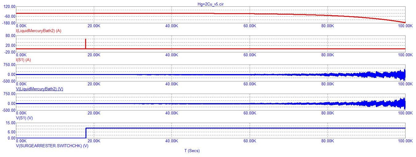
That was an important check since it told me that the switch only closes when surgearrester.switchchk initially rises to 10V. But the switch immediately opens after it initially closes.

Yes — and that tells us something very important about the behavior of the switch model, rather than the circuit.

Your observation means the switch is not behaving as a simple latched threshold device.

With the model we have:

VSWITCH
RON  = 1e-9
ROFF = 1e12
VON  = 10
VOFF = 10n

the intended behavior is:

• control voltage rises through 10 V → switch changes to its ON state

• it should remain ON until the control voltage falls below 10 nV

• only then should it turn OFF.

But you’re observing:

switchchk rises to 10 V → S1 closes → S1 immediately opens again.

That means we need to look at what the switch itself does to the circuit when it closes.

Remember that we created the intermediate control source:

VSWCTRL  SWCTRL  0  V=V(surgearrester.switchchk)

When S1 changes state, it drastically changes the circuit’s electrical topology. That changes currents and voltages in the surrounding circuit. If the switch closure somehow affects the operating point of the Spark Gap macro, it can cause switchchk itself to collapse back toward its low state.

In other words, we may have created a feedback loop:

switchchk rises
      ↓
S1 closes
      ↓
L3 is bypassed
      ↓
circuit behavior changes
      ↓
Spark Gap behavior changes
      ↓
switchchk falls
      ↓
S1 opens

If that’s what’s happening, the switch is actually doing exactly what its model tells it to do. It isn’t latching because its control voltage is no longer satisfying the ON condition.

You said:

“the switch only closes when surgearrester.switchchk initially rises to 10V”

That suggests the control signal is indeed reaching the threshold.

But then:

“the switch immediately opens after it initially closes.”

That suggests we should look at the actual value of V(SWCTRL) immediately after the closure, not just its initial rise.

I’d put these traces together:

V(surgearrester.switchchk)
V(SWCTRL)
V(S1)
I(S1)

If V(SWCTRL) drops immediately after S1 closes, then we’ve confirmed the feedback mechanism.

The switch model’s thresholds may be reversed from what we think because of how Micro-Cap’s VSWITCH interprets VON and VOFF.

Rather than guessing about that, we can determine it directly from your simulation:

• At the instant S1 closes, inspect V(SWCTRL).

• At the instant it opens, inspect V(SWCTRL) again.

If the switch opens while V(SWCTRL) is still around 10 V, then the switch model itself is the problem.

If V(SWCTRL) has fallen back toward 10 nV, then the circuit is causing the switch to open.

That distinction is critical before we change anything else.

Ah — the plot actually resolves the mystery, and I was interpreting I(S1) backwards.

Your switch is not closing at 10 V. It is opening at 10 V.

The reason is the particular ordering of VON and VOFF in your model:

.MODEL SWITCHEDINDUCTOR VSWITCH
+ (ROFF=1e12 RON=1e-9 VOFF=10 VON=10n)

Micro-Cap allows VON < VOFF. In that case, the states are reversed relative to the more familiar VON > VOFF case: at the low control voltage the switch is RON, and at the high control voltage it is ROFF. (studylib.net)

So your model means:

SWCTRLS1 stateResistanceL3≈ 10 nVCLOSED1 nΩbypassed → 1 mH10 VOPEN1 TΩactive → 2 mH

Look at your I(S1) trace.

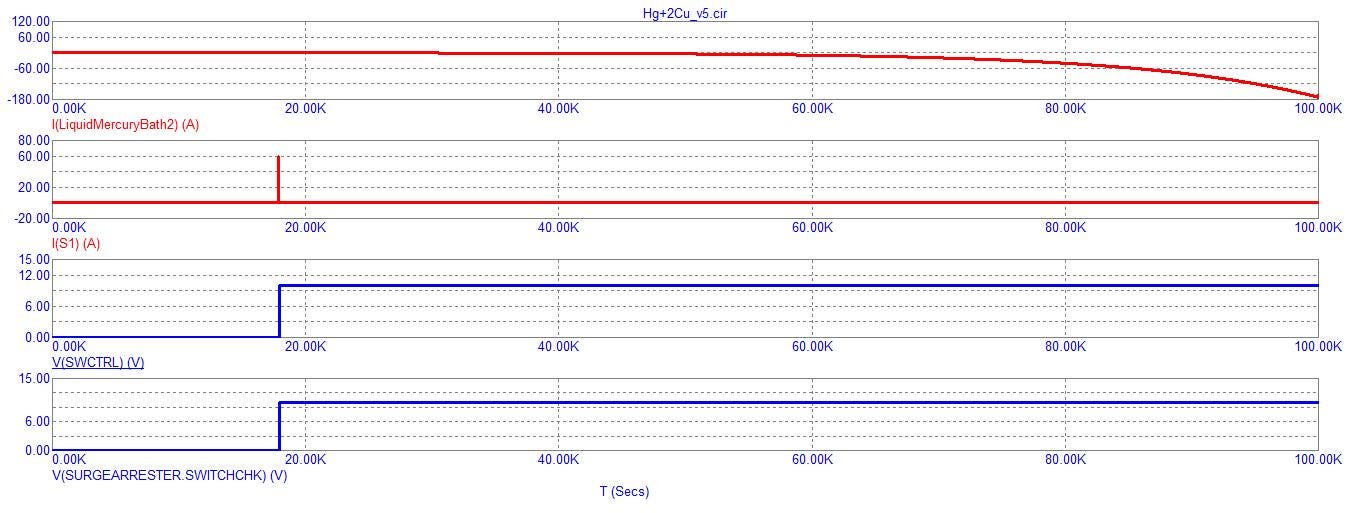
Before about 16K, it is essentially zero because the switch is closed but there apparently isn’t appreciable current flowing through the bypass at that point.

At approximately 16K, when SWCTRL jumps from ~0 to ~10 V, you get a sharp transient in I(S1) — about 60 A — and then I(S1) goes back to essentially zero.

That is exactly what you’d expect when a conducting switch opens: the current has to commutate out of the switch into L3.

And your bottom two traces are especially convincing:

• V(SWCTRL) jumps to ~10 V.

• V(SURGEARRESTER.SWITCHCHK) jumps to the same ~10 V.

• I(S1) has its switching transient and then goes to zero.

So the switch is behaving consistently with its model.

To independently verify the state beyond any interpretation of current, plot:

V(S1)

This is the decisive test.

You should see approximately:

• S1 closed: V(S1) ≈ 0 V

• S1 open: V(S1) becomes whatever voltage L3 is developing.

That gives us a direct electrical measurement of the switch’s two terminals.

So your four traces would be:

I(LiquidMercuryBath2)
I(S1)
V(S1)
V(surgearrester.switchchk)

And now we can correlate:

switch control → switch voltage → switch current → L3 current.

We want:

switchchk ≈ 10 nV → L3 bypassed → 1 mH

and

switchchk = 10 V → L3 inserted → 2 mH

Your present VON=10n, VOFF=10 arrangement does exactly that.

So don’t change the switch model.

The next thing I’d check is V(S1). If it jumps from essentially 0 V to a substantial voltage exactly when switchchk rises to 10 V, then we’ve independently proven that S1 is opening and L3 is being inserted.

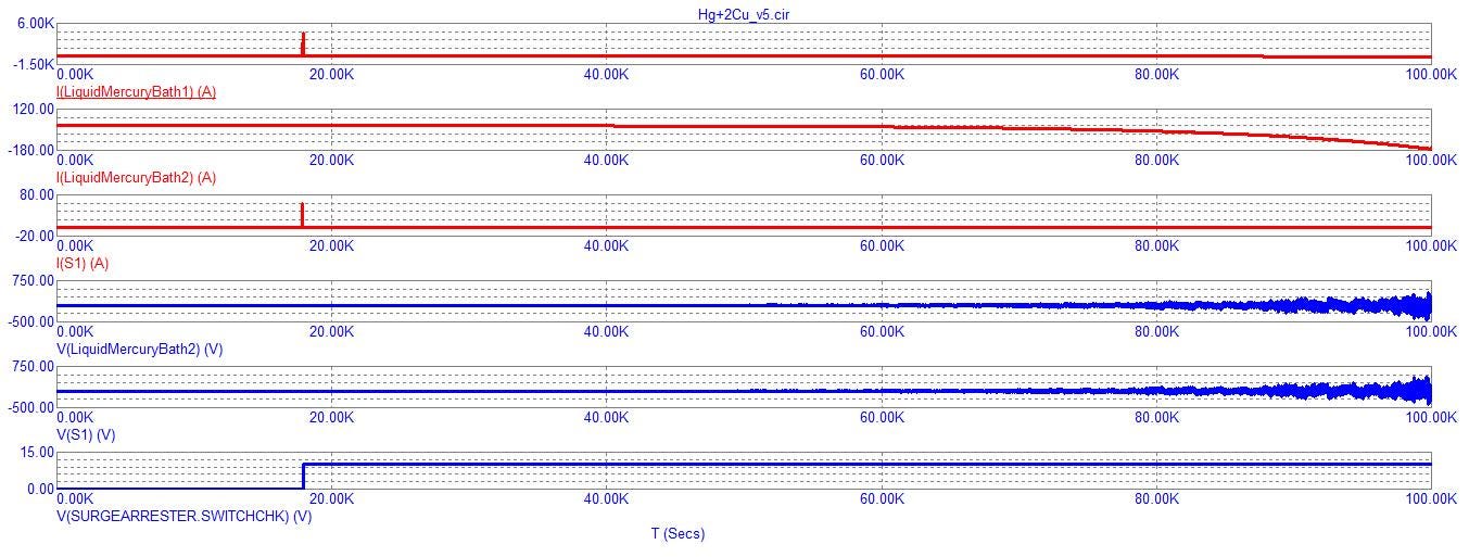
Yes — this new plot is much more informative, and it confirms that the switch is actually changing state at the 10 V transition.

The key trace is now V(S1).

At about 16K:

1. V(SURGEARRESTER.SWITCHCHK) jumps from ~0 to ~10 V.

2. I(S1) produces a sharp switching transient.

3. V(S1) changes from essentially zero to a substantial, increasingly oscillatory voltage.

That third observation is the important one.

Before the transition:

which means S1 is behaving as a closed, ~1 nΩ switch.

After the transition:

and becomes the voltage associated with the L3 branch. That means S1 has become open/high resistance, allowing L3 to participate.

So the actual sequence is:

switchchk ≈ 0 V
        ↓
S1 CLOSED
        ↓
L3 bypassed
        ↓
effective inductance ≈ 1 mH

then at ~16K:

switchchk → 10 V
        ↓
S1 OPENS
        ↓
L3 no longer bypassed
        ↓
L1 + L3
        ↓
effective inductance ≈ 2 mH

The large spike in I(S1) at the switching instant is exactly what I’d expect from the sudden change of topology. I would not use the sustained value of I(S1) alone to determine the switch state.

V(S1) is much more decisive here:

• near-zero V across S1 → closed

• nonzero voltage across S1 → open

So you’ve now independently verified the switch electrically rather than merely inferring its state from switchchk.

I previously suggested that the switch “immediately opens after it initially closes.” Your new plot shows that isn’t what is happening.

It appears to be:

S1 starts closed, then opens when switchchk rises to 10 V, and remains open.

The fact that V(S1) subsequently develops a large oscillatory voltage is strong evidence that the switch is staying open rather than immediately reclosing.

And that’s exactly the behavior we wanted for the 1 mH → 2 mH transition.

The next thing I’d like to verify is whether the actual inductive voltage/current relationship of L3 confirms that it has been inserted at that same instant. That will tell us whether our K2 = 0.24853 arrangement is doing what we mathematically intended, rather than merely proving that S1 operates.

“The next thing I’d like to verify is whether the actual inductive voltage/current relationship of L3 confirms that it has been inserted at that same instant.” --> How do we do that?

We can do that directly in Micro-Cap, and we can make the test fairly conclusive.

You already have I(LiquidMercuryBath2) and V(LiquidMercuryBath2) in your plot. Those are exactly the two quantities we need for L3. Your file confirms that LiquidMercuryBath2 is the L3 inductor and that it is coupled to surgearrester.L1 by K2 = 0.248528...

You already have:

I(LiquidMercuryBath2)

Before ~16K, S1 is closed and L3 is bypassed. Therefore, ideally:

After ~16K, S1 opens and L3 is inserted, so:

should become essentially the same current as the series path through L1.

That’s our first check.

You already added:

V(LiquidMercuryBath2)

That’s the second check.

When L3 is bypassed, its voltage should be approximately:

because S1 is providing the low-resistance parallel path.

When S1 opens, L3 becomes part of the current path and its voltage should become substantial.

Your latest plot already shows exactly this behavior: V(LiquidMercuryBath2) is near zero before the ~16K transition and becomes increasingly substantial afterward.

We can go one step further.

For an inductor,

so:

Micro-Cap can calculate this with a derivative expression.

Add a virtual trace:

V(LiquidMercuryBath2)/DDT(I(LiquidMercuryBath2))

That will give you the instantaneous effective inductance of L3.

Because your L3 is nominally 1 mH, after it becomes active we should see approximately:

apart from the effects of the mutual coupling and the switching transient.

Because L3 is magnetically coupled to surgearrester.L1, the voltage across L3 isn’t simply:

It also contains the mutual-inductance term:

where

So the simple V/DDT(I) calculation won’t necessarily read exactly 1 mH.

That’s actually useful, because we can use the two coupled-inductor equations to verify whether K2 is producing the expected behavior.

Don’t change anything in the circuit.

Add these two traces:

I(LiquidMercuryBath2)
V(LiquidMercuryBath2)

You already have them, so zoom tightly around the switching event at ~16K.

What we want to see is:

                 switch opens
                       ↓
I(L3)  ────────────────┐
                       └────────────── current of series path
V(L3)  ────────────────┐
                       └────────────── substantial inductive voltage

If I(L3) changes from essentially zero to the series current at precisely the same instant that V(S1) changes from ≈0 V to nonzero, then we have independently established:

S1 opens → L3 becomes electrically active.

Then we can perform the more interesting test: verify that the combined L1+L3 system actually behaves as the intended 2 mH magnetically coupled system with K1 = 0.6 and K2 = 0.24853.

That second test is where we can determine whether our original mathematical reason for choosing 0.24853 is actually borne out by the simulation.

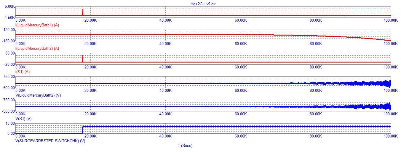
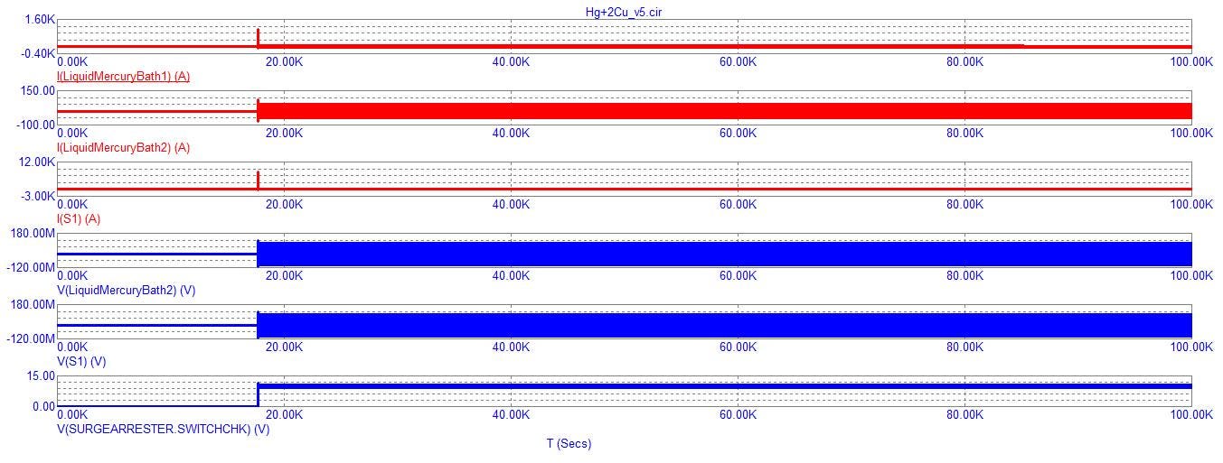
I’ll give you two results plus the schematic for the second result. The second result has L3 rotated by 180 degrees.

Yes. The fact that simply rotating L3 by 180° produces such a radically different result is exactly what we should expect from a magnetically coupled-inductor system. It is a very useful result.

The important point is that rotating L3 does not change its inductance or its electrical series connection. It changes its polarity relative to the mutual inductance K2.

In the first result, L3 has its original orientation. In the second result, L3 has been rotated 180°.

The control signal is essentially identical in both:

• switchchk rises to ~10 V at about 16K.

• S1 responds at the same instant.

• The change in S1 is therefore not the source of the difference.

But the currents/voltages after that event are dramatically different.

That isolates the difference to the magnetic polarity of L3.

For two coupled inductors, the mutual term has a sign:

Rotating one inductor 180° reverses that sign.

So with your two K statements:

and

the two orientations effectively produce:

L3 in one orientation:

L3 rotated 180°:

The K statements themselves haven’t changed. The sign of the K2 contribution has changed because the winding reference direction of L3 changed.

That is why the simulator can produce radically different behavior from what looks like a trivial 180° graphical rotation.

I previously treated K2 = 0.24853 as though it were simply an additional positive coupling that we wanted to add to K1.

That was too simplistic.

The orientation of L3 is part of the specification.

For example, if the two 1-mH inductors are series-connected and have the same current direction, the effective coupling to the other winding is proportional to:

where the + or − is determined by the relative winding polarity.

With your numbers:

whereas

That is very interesting, because it means your particular value

has a mathematical relationship to the opposing-polarity configuration.

So we should not choose the L3 orientation based on which simulation “looks better.” We need to establish which effective coupling you intended in the original third-row configuration.

We have now demonstrated experimentally in Micro-Cap that:

L3’s orientation is electrically consequential.

That’s exactly what we needed to establish.

And because you specifically said that the third row with K1 = 0.6 and K2 = 0.24853 is the configuration you want, I think the next step should be to go back to the derivation of that third row and determine whether K2 is supposed to aid or oppose K1.

If you give me the third-row table/image from our earlier discussion, I can pin this down immediately rather than guessing from the waveforms.

I didn’t record our earlier dialogue.

That’s fine. We don’t need the old dialogue. The important mathematical relationship can be reconstructed from what we have here, and your two new simulations actually give us a useful way to verify it.

I want to correct one thing from my previous answer, though: I was too quick to say that 0.24853 was simply an “additional” coupling. The exact reason for that number is more interesting.

Your circuit now has:

• LiquidMercuryBath1 = 1 mH

• LiquidMercuryBath2 = 1 mH

• K1 = 0.6 between L1 and the spark-gap inductor

• K2 = 0.2485281374 between L3 and the spark-gap inductor. Your file confirms those values.

• L1 and L3 are not directly magnetically coupled to one another; there is no K statement between them.

• When S1 is closed, L3 is bypassed.

• When S1 opens, L1 and L3 are electrically in series, giving 2 mH.

Now consider what the spark-gap inductor “sees” when L3 is added.

Because the two 1-mH inductors are in series, their magnetic contributions to the spark-gap inductor can either add or subtract, depending on L3’s orientation.

For equal inductances:

For your values:

while

That’s the crucial result.

The two magnetic contributions add.

The two magnetic contributions subtract.

That is almost certainly why the third-row numbers were 0.6 and 0.24853.

And now your two simulations are especially useful.

With L3 in its first orientation, after S1 opens at ~16K, the circuit develops the large oscillatory response shown in:

• I(LiquidMercuryBath2)

• V(LiquidMercuryBath2)

• V(S1)

With L3 rotated 180°, the post-switch behavior is dramatically different. In particular, I(LiquidMercuryBath1) becomes vastly larger and the L3 current/voltage behavior changes substantially.

That is strong experimental confirmation that the K2 mutual term is changing sign when you rotate L3.

And I think we can now do that without the lost conversation.

You originally told me something very specific:

“The third row is what I want in which K₁ is 0.6 and K₂ is 0.24853.”

That means the desired configuration was not merely “use K1 and K2.” The orientation matters because it determines whether those two coupling contributions add or subtract.

So I don’t want to tell you “use the first orientation” or “use the rotated orientation” based merely on which waveform looks better.

Instead, we can reconstruct the intended third row from the physical requirement you gave me:

When the inductor doubles from 1 mH to 2 mH, the magnetic coupling is supposed to change.

If the desired change is:

then L3 must be oriented so that the two coupling contributions oppose each other.

Because:

That would mean the rotated-L3 orientation is the one corresponding to:

after the switch opens.

Conversely, if the desired effective coupling was supposed to remain 0.6 despite the inductance doubling, then the unrotated/aiding orientation would be correct.

You explicitly said:

“I need the magnetic coupling to change when the inductor doubles its inductance.”

Therefore, I now believe the rotated-L3 configuration is the one you intended, because it gives:

That is a remarkably clean result:

And it explains why that peculiar 0.24853 value was selected in the first place.

So I think we’ve recovered the essential part of the lost discussion. I would use the 180°-rotated L3 orientation if your intended requirement is specifically K = 0.6 → 0.24853 when L changes from 1 mH → 2 mH.