Lecture 2: The Economy and the Environment

Last week I promised that this lecture would cover why markets are good, why they fail, and what role government plays. This post addresses those issues at the 30,000-foot level. Recognizing that a full semester course could be devoted to each of these sections, the goal here is not to become an expert but rather to get a familiarity with concepts that will show up over the course of the semester. I want to flag up front that I built a web tool to help understand the Coase Theorem — please check it out later in this post.

The market effects of a policy are not always obvious. A few examples: building LNG terminals in the US leads to increased natural gas prices domestically (DOE, 2024); donating used clothing to developing countries can be a net negative as it competes with the local textile industry as well as leading to pollution from the discarded clothes (Frazer, 2008); putting tariffs on steel leads to an offsetting decline in domestic manufacturing (Flaaen and Pierce, 2019). Thinking through the ramifications of policymaking will be a theme throughout this class, and economics is one of the key frames of reference for understanding those ramifications (though not the only one!).

The main framework for federal regulatory analysis in the US is OMB Circular A-4. I’ve written about it before; here is the short version, starting with the history:

• 1981: EO 12291 established the requirement for regulatory impact analysis for “major rules.”

• 1993: EO 12866 (pdf) added more process detail and transparency requirements.

• 2003: OMB Circular A-4 provided guidance for all aspects of cost-benefit analysis.

• 2023: The revised OMB Circular A-4 (pdf) updated and improved many aspects of the 2003 doc, particularly discounting, EJ, and global aspects.1

• 2025: Trump directs the OMB Director to revoke the 2023 Circular A-4 updates.2

What can we learn from OMB Circular A-4? Three things:

1. The justifications for regulation (correcting market failures or serving other social purposes).

2. Guidance on regulatory design and how to do cost-benefit analysis (which alternative provides the largest benefit to society?) or cost-efficiency analysis (which alternative most efficiently achieves a given goal?). Both compare a future world “with the policy” to a “no-policy” baseline. Defining the right baseline is important both in economics and in climate science.

3. A preference for market-based regulatory approaches (contrast with ecological economics, where market mechanisms are not the primary framing).

Textbook free markets rely on some strong assumptions:

• Perfect information

• Perfect or complete competition (i.e., no single entity can influence prices)

• Clear and complete property rights

• No transaction costs

• No externalities

• Rational behavior

Given these assumptions, markets yield a welfare-maximizing and “Pareto-optimal” outcome: this means that you can’t make the pie bigger, and you can’t make any individual party better off without making another worse off. (Note: this does not yet touch the distribution of that welfare.)

The core concept is supply and demand. A supplier is willing to sell more units as price rises; a consumer is willing to buy more units as price falls. The market clears where they meet (Figure 1). The area above the price and below the demand curve is consumer surplus: the value the consumer gets above what they paid. The area between the price and the supply curve is producer surplus: the revenue the producer receives after production costs (not taking into account fixed costs). Total surplus is maximized at the equilibrium. The division of surplus between consumers and producers depends on the shape of the curves and can be shifted by tactics like coupons, age discounts, micro-charges, or one-day sales. The potential for surveillance pricing (FTC, 2025) in a world with AI is particularly worrisome here.3

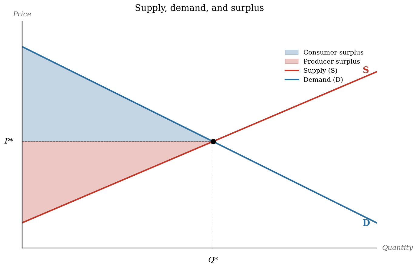
Figure 1: Supply and demand with consumer and producer surplus. Total surplus is maximized where S = D at (Q*, P*).

Two related concepts:

Production possibilities frontiers. Say you’re growing herbs on your balcony. You can plant basil (which likes sun) or mint (which likes shade), and there’s a frontier of what’s achievable given your balcony’s geometry. If you’re inside the frontier, you can grow more of either. If you’re on the frontier, you can’t grow more of one without growing less of the other. That’s the production possibilities frontier: a state where it isn’t possible to make more of one thing without making less of another. But it makes no statements about whether any one place on the frontier curve is better than another. A parallel concept is Pareto optimality, but applied to welfare across people rather than production across goods.

Elasticity. How much does quantity change when price changes? Insulin is nearly perfectly inelastic: demand doesn’t change much no matter the price, because you need what you need. At the other end, for an individual seller, the demand curve is perfectly elastic (e.g., one farmer can sell as much of their Number 2 Winter Wheat as they want without the price dropping4) (Figure 2). Most real goods are somewhere in between. Elasticities can also shift over time: gasoline demand is inelastic in the short term (you have to drive to work) but elastic in the long term (you can move closer to work or buy a more efficient car).

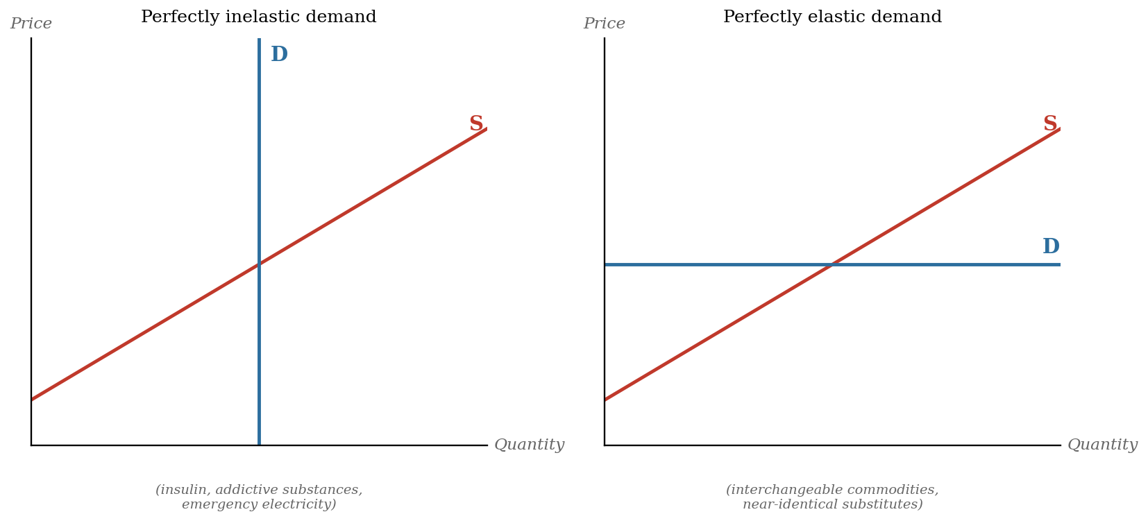
Figure 2: Two extremes of elasticity of demand — perfectly inelastic (vertical) and perfectly elastic (horizontal).

Finally, decisions should be made at the margin. If the marginal benefit of the next unit exceeds its marginal cost, produce more. If it’s less, produce less. The optimum is where they meet. This principle drives cost-benefit analysis.

But as telegraphed in the last section, market efficiency assumptions can be unrealistic. Modes of failure include:

1. Externalities (pollution)

2. Information asymmetries (used cars)

3. Monopolies (electricity grid)

4. Non-rational behavior (inconsistent internal discount rates)

5. Principal/agent (e.g., tenant/landlord, realtors, …)

We will go deeper on the first three failures here, and then cover a couple more relevant concepts.

Externalities. This is the market failure that is most relevant for climate policy. Suppose producing a widget causes $5 of pollution damage to third parties. The producer doesn’t pay that $5, so their private cost of production is less than the social cost. The consumer doesn’t pay that $5 either. The market equilibrium delivers more widgets than is socially optimal, with the social cost of that overproduction equal to the deadweight loss (Figure 3).

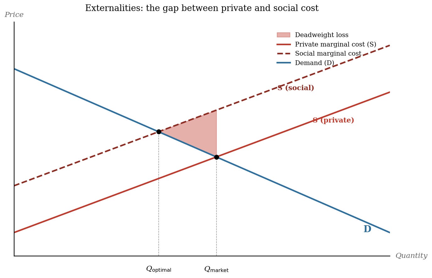
Figure 3: When there is an externality, private cost is lower than social cost. The market produces at Q_market rather than the socially optimal Q_optimal, and the shaded triangle is deadweight loss.

Monopolies. Monopolies can result in higher prices and/or inferior products without the pressures of competition (though higher profits can also mean investment in R&D, as in the era when AT&T monopoly profits funded Bell Labs (Gertner, 2012, The Idea Factory), leading to the invention of the transistor). Natural monopolies like electricity distribution require careful regulation, but the intersection between regulated markets and free markets can be fraught (Enron made big bucks in 2000 manipulating the partially deregulated California market, as detailed in Borenstein, 2002).

Information asymmetries. The classic asymmetric example is used car markets (Akerlof, 1970, pdf). Sellers know if the car is a lemon; buyers don’t. Solutions include lemon laws (a government approach) or warranties and inspections (a market approach).5 Inadequate information (as distinct from asymmetric information) can be addressed by minimum standards (e.g., stroller safety) or labeling requirements (see Figure 4 as an example of how the government can require car manufacturers to provide mileage information in a way that will be most useful to consumers).

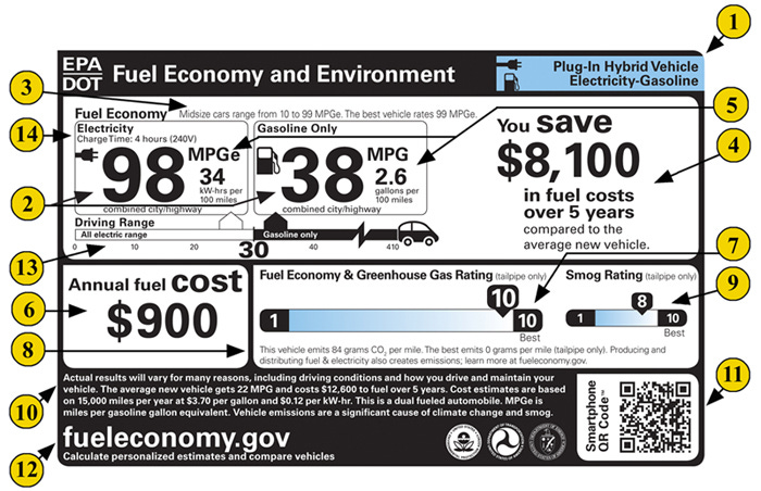
Figure 4: EPA/DOT Fuel Economy label for plug-in hybrid vehicles.

Public vs. private goods. Two questions about a good: is it rival (does one person’s use either prevent another person’s use or degrade the good, reducing its desirability)? Is it excludable (can non-payers be prevented from using it)?

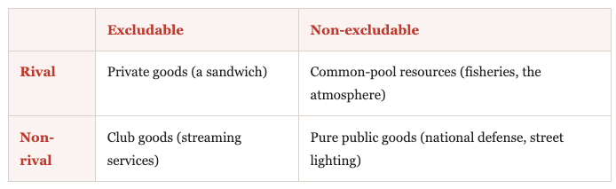
Table 1: Different types of goods. See Figure 1 in Elinor Ostrom’s 2009 Nobel Lecture (pdf).

Free markets are usually well-suited to optimize production of private goods. For everything else, there’s a potential role for government intervention.

The Coase theorem. In 1960, Ronald Coase argued that if property rights can be clearly assigned, then regardless of who holds the rights, the same outcome will be reached through bargaining (setting aside transaction costs). He chose Sturges v. Bridgman (1879) as an example, where a doctor sued a confectioner whose noisy mortar-and-pestle disrupted his consultations. The court ruled in favor of the doctor. Coase’s idea was that whether the default right was to quiet or to being able to make noise, money could be exchanged in order to reach an optimal outcome. Moreover, that optimal outcome would be the same either way (though who ended up with the money would differ). This is the fundamental idea behind cap-and-trade: regardless of whether permits are allocated to industry for free, or held by the government and sold, the emissions outcome should be the same.6 Coase doesn’t apply as well when there are large transaction costs (e.g., if you need expensive monitoring to figure out what’s going on) or large numbers of participants (too much incentive for free riding).

I have tried to work out the Sturges v. Bridgman example on a white board, and it didn’t go well. However, I have now created a Coase Theorem online learning tool. Please test it out and give me feedback as to whether this helps understand property right allocation and/or marginal cost curves.

If externalities are the market failure, how can we fix it?

Pigouvian taxes. Add a tax equal to the marginal external damage.7 The tax internalizes the externality, thereby enabling the market to reach the socially optimal quantity.

Quotas. Determine the optimal emission quantity. Create a number of permits equal to that quantity. Let the market determine the optimal price.

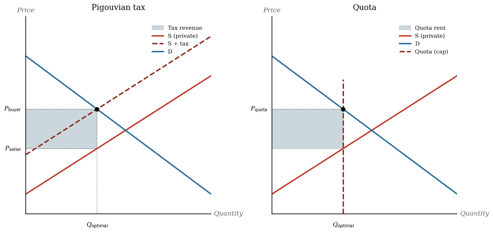
Figure 5: Two ways to correct an externality. Left: a Pigouvian tax equal to the external damage shifts the supply curve up. Right: a quota caps the quantity at the same point. Both reach Q_optimal under textbook conditions.

In theory, the optimal tax or the optimal cap and trade policy will end up with the same price and the same quantity emitted. However, if there is uncertainty in the supply or demand curves, the two approaches begin to differ, as the tax lets the quantity change to clear the market, whereas the cap and trade lets the price vary. There is an economic answer to which is more efficient depending on whether the slope of the marginal damage curve or the marginal abatement cost curve is steeper, which I will discuss in Lecture 5.8 There are also important political differences.

Two important questions about either approach:

1. Distribution. How is the revenue allocated? Are permits freely given or sold?

2. Valuation. Setting a price or setting a cap requires information about the damages caused by the emissions. How much is the marginal external damage worth in the first place? We will discuss this issue in Lecture 4.

Sometimes, government is the answer, and sometimes, it is the problem. Some modes of government failure include:

• Deadweight losses. Taxes that aren’t fixing an externality make for a less efficient market.

• Administrative burden. Paperwork or delays (or uncertainty) due to permitting are both costs to the economy.

• Regulatory capture. Rich companies often influence policymaking in their favor (see the Minerals Management Service in the 2000s, where drugs and sex were part of the influence operation).

• Barriers to entry. Some licensing requirements make sense, but sometimes they just exist to protect incumbents at the expense of new entrants. (The Louisiana florist licensing requirement was my go-to example, but apparently that was finally eliminated in 2024.)

• Perverse incentives. Mexico City’s Hoy No Circula rule, which barred cars from driving on certain days based on license plate numbers, led households to buy second (often older, dirtier) cars to drive on the restricted days (Davis, 2008, pdf).

• Anti-market regulations. Price controls and production quotas (as distinct from emission quotas on pollution) generally do more harm than good.

This is not an argument against most government regulation, it is an argument for intelligent policy design (okay, and an argument against unnecessary regulation).

All of this is complicated. How do economists think through this? Sometimes they use simple equations and diagrams (as in the Econ 101 section). But sometimes they build computer models that embody many of the key economic relationships to test how a policy might percolate through the economy.

Two broad approaches:

Top-down (general equilibrium). Model the whole economy as a system of interconnected markets. Prices adjust endogenously.9 These models include terms for goods, capital, labor, international trade, taxes, and other large scale economic issues… but tend to be sparse in terms of carrying a lot of different technological options.

Bottom-up (partial equilibrium). These models often focus on a single sector or set of sectors, and assume the rest of the economy stays constant. This allows for much more technological detail, but misses some of the ways that the larger economy can adjust to compensate.

Some economic models that I’ve used over the years include MOVES for vehicle emissions, the EPPA CGE model for whole economy modeling, the GCAM model for partial equilibrium modeling, and GIVE and FrEDI for estimating damages. Other popular models include the power sector models like NEMS or IPM, and the global damage models that were used for the Obama SC-GHG (TSD pdf) (DICE, FUND, PAGE).

All economic models have limitations. We will likely (hopefully?) never reach the predictive capabilities of Asimov’s psychohistory.10 What the world will look like decades in the future will depend on which technologies are developed, how human preferences shift, and other changes we can’t predict… and yet, despite all the crazy history over the past century, if we look at global GDP it has been pretty smooth. So economists do their best to use historical patterns to figure out what plausible futures might look like. There may not be underlying physical laws like in climate models, but the alternative to making our best guess is to assume we know nothing about what the future might look like, and then how could we ever make any decisions at all?

Next up: the Carbon Economy — where our emissions actually come from, and how we project where they’re going.