The state vector and the Measurement Postulate- Book Excerpt #19

This is section III.4 (that builds upon the previous section here) of the first volume of my book, “Quantum Physics: An Overview of a Weird World.” I plan to post regular updates, including minor and substantial revisions, on Substack. Here is the full table of contents and guidance on how to follow the book as it unfolds.

We have seen that QM is a purely probabilistic theory. Accordingly, events occur only with a certain probability but the single event can never be predicted with certainty unless the system is already prepared into a state called an eigenstate—that is, that kind of quantum state in which repeated measurements of the quantum system will always lead to the same result.

Yet, in general, quantum events are purely random and we must resort to statistical reasoning and predictions as well as a statistical formalism and math. This is essentially what distinguishes CP from QM, the purely probabilistic and random nature of the latter.

As we already mentioned with Laplace’s demon, in CP, if you fix the boundary conditions, a system will always evolve in the same manner, and it is deterministic and predictable, at least in principle. In QT, even if you shoot the particles from the same place, with the same speed toward the very same slits, you will always see them lighting up a different spot on the detection screen.

However, this does not mean that nothing can be said about the average behavior of a system, say, a system of particles, or its dynamic and temporal evolution. In this case, it is perfectly possible to describe it according to some statistical rules—for example, the statistics that describe the distribution of a large number of particles on a screen according to an interference fringes pattern. This also means that, in QM, the math describing the dynamics of a physical system must be very different. Instead of ascribing to a particle a single final possible state, one must resort to the wave function, which describes several possible measurement outcomes probabilistically, though the particle’s initial condition is known. Let us, therefore, go through a (not at all rigorous) brief introduction to some formal aspects of QM. I will try to keep it a intuitive-friendly introduction in contrast to a complete course on QM but it is nevertheless necessary to digest some simple yet very important formalism and symbolism, as it will continue to emerge frequently here and there, and it is that kind of representation that you will encounter throughout all textbooks on QM. Therefore, this section assumes familiarity with basic mathematical concepts such as vector spaces, complex numbers, and elementary algebra.

So, let us turn our attention back to the concept of the wave function. We considered it to be continuous for the position in space of a particle, and its value, the probability density or the integrated probability function of the particle in space, does not change abruptly from one point to another. That is, the wave function ψ(x) is a continuous function in x.

We saw, however, that there can be other behaviors of quantum systems—for example, the energy state of atoms is quantized. Here, the wave function can no longer be a continuous function but must be represented by a set of discrete possible states of the system—for instance, as we have already seen in the case of the hydrogen spectrum or in the Franck-Hertz experiment. In these cases, we are dealing with a different physical context than that of a continuous spectrum of possible outcomes, such as that of a particle moving smoothly (i.e., continuously) along a spatial axis, but we must represent the quantum system’s states with a discrete spectrum—that is, the wave function ψ is not a continuous function in space but is a collection of a more general set of N distinct abstract states, so-called eigenstates (from the German “eigen,” which means “self”) e1, e2, .., eN , each standing for the system’s possible discrete states, here the energy levels E1, ..., EN . The same fits for other discrete dynamical variables, such as the position, the momentum, the angular momentum, the spin, etc., or other dynamical variables that are a combination of these physical quantities.

Notice that N , the total number of possible states a system can assume, may be either finite or infinite. For example, as we shall see, the quantum spin of a particle can take only two possible states (N = 2), whereas an unconstrained particle in a continuum can, in principle, occupy infinitely many position states (N = ∞). However, keep in mind that an infinite number of possible states does not necessarily imply a continuous spectrum. For instance, as illustrated, the energy levels of the hydrogen atom are infinite in number, yet the spectrum is discrete. This is because the higher energy levels accumulate, with the spacing between successive levels becoming arbitrarily small.

In QM, these eigenstates are defined on a Hilbert space. Without going too much into mathematical details, it suffices to say that a Hilbert space is an abstract vector space that is an extension of the real Euclidian space to a multidimensional space of complex numbers and complex vectors. If the Hilbert space has a finite dimension, it is the state space of a quantum system with a finite number of eigenstates. Otherwise, it is infinite—as infinite as the number of its degrees of freedom. Another important difference in a “space” as we conceive of it in school geometry is that the elements of a Hilbert space are no longer points and coordinates but, rather, vectors or functions, with the wave function being the primary object on which to act. A Hilbert space is essentially an extension of the Euclidean space from a real to complex vector space and with a well-defined notion of distance and angles.

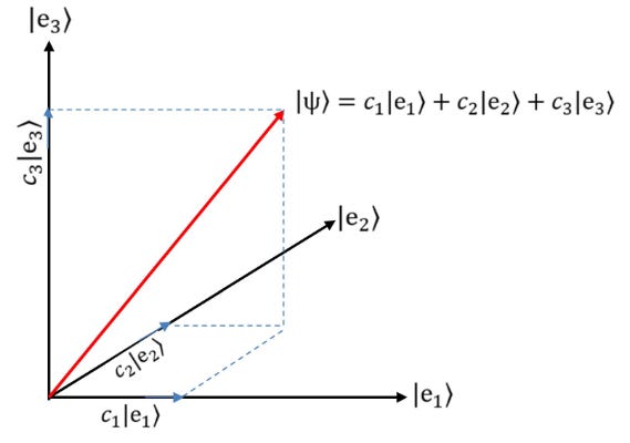
The eigenstates e1, e2, .., eN , form the eigenbasis of the Hilbert space, and the overall possible states of a quantum system are represented by a vector defined on this eigenbasis, called the state eigenvector, or just eigenvector, or simply the state vector (in Fig. 1 a simple case for a system with three possible eigenstates is shown):

where c1, c2, .., cN , are complex coefficients which are calculated and interpreted as follows.

Consider the orthonormal eigenstate vectors |e1⟩ , |e2⟩ , .. |eN ⟩. Geometrically, this is displayed in Fig. 1 as being all these eigenstate vectors perpendicular (with unity length) to each other.1 Physically, this means that one or the other state can be measured, though never more than one at a time. Orthogonality implies mutually exclusive measurement outcomes.

Because we are no longer dealing with a continuous function but, instead, with a state vector in which each element corresponds to discrete eigenstates (think again of the eigenenergy spectrum of the hydrogen atom), the probability density function (Eq. 1 here) must also be replaced by discrete probabilities. In general, the probability of finding the system in one or another eigenstate is not the same. For example, the probability P1 of finding the Hydrogen atom in an energy state E1 is not the same probability P2 of finding it in a state E2, etc. That’s why the spectral lines have different thicknesses, that is, intensities. Nonetheless, the set of all probabilities P1, P2, .., PN must sum up to unity—that is, certainty that the system will be found in at least one among all the possible states.

Formally this information regarding with what probability each of the eigenstates will be observed after a measurement is encoded in the complex coefficients c1, c2, .., cN , which determine the length of each eigenvector, as illustrated in Fig. 1.

This can be summarized in the Born rule, which still holds: The probability P associated with the i-th eigenstate ei is the squared modulus of the i-th complex coefficient ci :

The state vector notation |ψ⟩ of Eq. 1 is a common notation in QT. State vectors can be written according to the Dirac-notation. P. Dirac was a British physicist who made several contributions to QT.

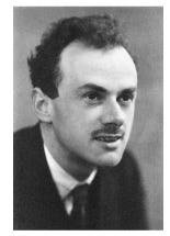
We already saw how the kind of notation for integrals we encountered as brackets, like ⟨a, b⟩, turns out to be a useful convention. Each bra-ket is a product of a “bra-vector” ⟨a| (a row vector whose elements are the complex conjugates of the vector elements of a) and a “ket-vector” |b⟩ (a column vector with the vector elements of b). As you can see, Dirac wasn’t lacking a bit of weird lexical fantasy, though this turned out to be extremely useful. For example, the general “bra-a, ket-b” is:

This is called an inner product and is just an extension of the familiar scalar product or dot product and that some might recall from their high school algebra, but extended to Hilbert spaces where vectors have complex entries. Never forget that if two vectors |a⟩ and |b⟩ are perpendicular (orthogonal), then ⟨a|b⟩ = 0, always.

With Dirac’s notation, many calculations are made formally simpler.

For example, consider the Hilbert space representation of the eigenvectors |ei⟩ relative to the eigenbasis (e1, e2, ..., eN ) and the state vector |ψ⟩ of Eq. 2, that is:

respectively.

Then the probability of finding the i-th eigenstate can also be written in the

bra-ket notation as follows:

Again, with the right-hand-side sum of all the modulus squared complex coefficients, each representing the probability of the i-th eigenstate to be measured, must obviously sum up to certainty (or, to put it another way, the sum of the probabilities of all possible events gives unity). Note also how the sum of all the probabilities adding up to unity is represented in Dirac’s notation neatly as:

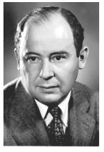
It is a symbolic formalism introduced by Dirac, and later developed further by others, such as the mathematician John von Neumann, with which one represents the probability of observing a system with a number of possible discrete states.

It is also customary to state that Eq. 5 is the modulus square of the projection of the state vector ψ onto eigenstate ei. In fact, the act of measurement, “projects” the state vector onto one of its eigenbasis vectors (one can interpret the dashed lines in Fig. 1 as “projections.”) This is analogous to the wave function collapse we saw in the case of a continuous wave function. There, the act of measurement “collapses” the wave function describing the particle position in a continuous space on one of the infinitely possible states. After all, the position of a particle is also a “state.” Here, it projects the state vector onto a discrete spectrum of possible eigenstates.

This description of quantum measurements derives directly from experimental observation and was first formalized by von Neumann, also known as von Neumann’s projection postulate, or von Neumann’s collapse postulate, which expresses the discontinuous, instantaneous and irreversible nature of the measurement process in QM.

In its modern version, it is also called the measurement postulate of QM, which states that:

i) For each measurement of a dynamical variable (or observable, see later on), the probability of finding it in one of its possible eigenstates is given by Eq. 5.

ii) After the measurement, the system instantly “collapses” from state |ψ⟩ to an eigenstate |ei⟩; (i = 1, .., N ).

iii) From that moment on, any new measurement will always show the system to be in the same eigenstate.

While this postulate has always been employed with success as a powerful predictive tool in QM, later on, we will see how it leads to some still-unsolved issues, summarized by the so-called measurement problem and famously represented by the Schrödinger’s cat experiment or paradox.

Moreover, once the quantum system has been placed into one of these eigenstates, in QM jargon one says it has been prepared into a specific state |ei⟩, and if it is not perturbed—that is, it does not interact with the environment suffering a state change—every subsequent measurement will always deliver the same result: the system being in state |ei⟩.

The next section will deal with operators and the Schrödinger equation.