Spatial Heterogeneity in Land Use Transition Probabilities

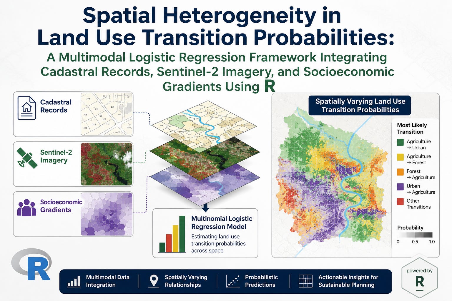
The article presents a complete R-based workflow for modelling spatial heterogeneity in land use transition probabilities using a multimodal multinomial logistic regression framework. The main purpose of the article is to show how different forms of data—cadastral records, Sentinel-2 style remote-sensing indicators, socioeconomic gradients and spatial variables—can be integrated into one interpretable statistical model to estimate how likely different parcels are to experience specific land use transitions.

The article begins by explaining that land use change is not spatially uniform. Parcels with similar initial land use may have very different transition probabilities depending on where they are located, how accessible they are, what planning zone they belong to, how much development pressure they face and what the surrounding socioeconomic conditions look like. For example, a vacant parcel close to a rail corridor may be more likely to become residential than a vacant parcel far from transport infrastructure. Similarly, a residential parcel close to a dense activity centre may be more likely to transition into commercial use than a residential parcel located in a low-density fringe area. This motivates the use of a spatially aware modelling framework.

The modelling problem is framed as a multiclass land use transition problem. Each parcel begins with an initial land use at time (t_0), such as agriculture, residential, commercial, industrial, vacant or green land. At a later time (t_1), the parcel may remain stable or transition into another category. The article defines six possible transition outcomes: stable, agriculture-to-residential, vacant-to-residential, residential-to-commercial, green-to-urban and industrial-to-commercial. Since the response variable has more than two categories, the article uses multinomial logistic regression rather than binary logistic regression.

The statistical framework is explained clearly. For each parcel, the model estimates the probability of belonging to each transition class conditional on a set of predictors. The predictors include cadastral, imagery, socioeconomic and spatial variables. The multinomial logistic regression model estimates separate coefficient vectors for each transition class relative to a reference class. In the article, the reference class is Stable, meaning that the estimated coefficients explain how each variable changes the relative log-odds of a specific transition compared with remaining stable. This makes the model highly interpretable, which is valuable for planning and policy applications.

A major part of the article is the creation of a simulated but realistic parcel-level dataset in R. The dataset contains 6,000 simulated parcels distributed across a hypothetical two-dimensional urban region. Each parcel is assigned x and y coordinates, a distance from the central business district, a spatial region, an initial land use category, zoning, ownership type, heritage status, parcel area, land value, accessibility measures, population density, income, Sentinel-2 style imagery indicators and land use transition outcome. Although the dataset is simulated, the relationships are designed to mimic realistic urban development processes.

The simulated cadastral variables include parcel area, land value, zoning, owner type, heritage flag and initial land use. These represent the kind of data commonly found in land administration or planning systems. For example, agricultural and green parcels are assigned larger parcel areas, while residential and commercial parcels tend to be smaller but may have higher land values due to accessibility and urban location. Zoning is linked to initial land use, with agricultural parcels commonly assigned rural, future urban or conservation zoning, and residential parcels assigned residential or mixed-use zoning.

The article also simulates Sentinel-2 style remote-sensing indicators. NDVI is used as a vegetation proxy, NDBI as a built-up intensity proxy, NDWI as a moisture or water-related proxy and red-edge as a vegetation condition proxy. These variables are designed to reflect the spectral differences between vegetated land, vacant land and built-up areas. Agricultural and green parcels tend to have higher NDVI, while residential, commercial and industrial parcels tend to have higher NDBI. This helps the model distinguish greenfield conversion from urban redevelopment.

Socioeconomic gradients are also simulated. Population density is highest near the urban centre and along transport corridors. Median income varies spatially, with some areas having higher simulated income and others having lower income. Rail access and road access are generated using spatial gradients and hotspot functions. These accessibility measures are then combined with population density and hotspot variables to create a composite urban_pressure indicator. This variable is important because land use transition is often driven by development pressure, infrastructure access and market demand.

The article uses spatial hotspot functions to create realistic spatial heterogeneity. For example, a north-east growth hotspot increases the probability of agriculture-to-residential transition, while a west industrial hotspot increases the probability of industrial-to-commercial transition. These spatial features make the simulated region more realistic because land use change tends to concentrate around corridors, nodes, redevelopment areas and growth fronts rather than spreading evenly across space.

The transition outcome is generated using a probabilistic mechanism. Each transition class has its own score, and these scores are converted into probabilities using a softmax function. Agriculture-to-residential transition is made more likely for agricultural parcels with high urban pressure, good rail access, future urban zoning and proximity to the north-east growth hotspot. Vacant-to-residential transition is made more likely for vacant parcels in accessible or residentially zoned areas. Residential-to-commercial transition is linked to residential parcels with high rail access, high density and built-up characteristics. Green-to-urban transition is more likely for green parcels under development pressure but less likely where heritage or conservation constraints are present. Industrial-to-commercial transition is linked to industrial parcels with strong road access and proximity to the industrial redevelopment hotspot.

The exploratory data analysis section is extensive and forms a major part of the article. It begins with a spatial map of baseline land use. This map shows how the initial land uses are distributed across the simulated region. Residential and commercial parcels are more concentrated around the urban centre and accessibility corridors, while agricultural and green parcels are more common in outer or environmentally sensitive areas. This figure demonstrates why spatial information is important in land transition modelling.

The second EDA figure maps the observed land use transition classes. This figure shows that transitions are spatially clustered rather than randomly distributed. Agriculture-to-residential transitions appear around growth areas, residential-to-commercial transitions occur near dense and accessible parts of the region, and green-to-urban transitions occur where development pressure is high but are partly constrained by heritage and conservation factors. This visual evidence supports the article’s central argument that transition probabilities are spatially heterogeneous.

The transition class distribution plot shows that most parcels remain stable, while transition categories are smaller. This reflects a realistic feature of land use change data: actual land conversion events are often relatively rare compared with stable land outcomes. The article highlights that this creates a class imbalance problem. In such settings, accuracy alone can be misleading because a model may perform well on the dominant stable class while doing poorly on smaller transition classes. This is why the article later includes macro F1 and class-level performance measures.

The cross-tabulation heatmap between initial land use and transition outcome validates the logic of the simulation. Agriculture-to-residential transitions mostly originate from agricultural parcels, vacant-to-residential transitions mostly originate from vacant parcels, residential-to-commercial transitions mostly originate from residential parcels, and industrial-to-commercial transitions mostly originate from industrial parcels. This figure is important because it shows that the simulated transition outcomes follow plausible land use pathways rather than arbitrary class assignments.

The EDA also includes boxplots of NDVI, NDBI and land value by transition class. The NDVI boxplot shows that green and agricultural transitions tend to have higher vegetation values, while built-up redevelopment transitions tend to have lower NDVI. The NDBI boxplot shows the opposite pattern, with built-up transitions having stronger built-up signals. The land value boxplot shows that redevelopment-oriented transitions are often associated with higher-value parcels, reflecting the economic logic of intensification in accessible and desirable locations.

Spatial surface maps of population density and urban pressure are also included. The population density map shows a typical urban gradient, with higher density near the central area and accessibility corridors. The urban pressure map shows where development pressure is strongest, combining the effects of accessibility, population density and growth hotspots. This figure is especially important because urban_pressure is a key explanatory variable in the transition model.

A correlation heatmap is used to examine relationships between numerical predictors. It helps identify associations such as the positive relationship between rail access, population density and urban pressure, as well as the negative relationship between NDVI and NDBI. This step is useful because highly correlated variables can affect model interpretation. The article does not remove these variables, but it uses the heatmap to make the relationships transparent.

The article then introduces feature engineering for spatial heterogeneity. In addition to raw x and y coordinates, it creates normalized coordinate variables, an x-y interaction term, NDVI-by-x interaction, NDBI-by-y interaction, income-by-access interaction and urban-pressure-by-NDVI interaction. These variables allow the model to capture the idea that the same predictor can have different implications in different parts of the region. For example, high NDVI in a protected green area may imply conservation stability, while high NDVI near a growth corridor may imply future urban conversion risk.

The modelling workflow uses a stratified train-test split with the caret package. Numerical variables are scaled using statistics from the training data, and the same scaling is applied to the test data. This is an important modelling practice because it avoids data leakage from the test set into the training process. The multinomial logistic regression model is then fitted using nnet::multinom. The formula includes all numerical, categorical and engineered spatial interaction variables.

The model prediction section generates both predicted classes and predicted probabilities. This distinction is important. Predicted classes assign each parcel to the most likely transition outcome, while predicted probabilities show the model’s estimated risk for each possible transition. For planning applications, predicted probabilities are often more useful than hard classifications because decision-makers may need to prioritize parcels based on risk thresholds.

The article evaluates model performance using accuracy, macro F1 and multiclass log loss. Accuracy measures the overall proportion of correct predictions. Macro F1 gives equal weight to each transition class, making it more useful when the outcome is imbalanced. Log loss evaluates the quality of predicted probabilities. The inclusion of log loss is especially valuable because land use transition modelling often depends on reliable probability estimates rather than only correct class labels.

A classification report is created manually in R. It provides precision, recall, F1 score and support for each transition class. This allows the reader to examine whether the model performs well across all classes or mainly on the dominant stable class. The confusion matrix then visualizes observed versus predicted classes. It helps identify which transition types are commonly confused and whether rare transitions are being misclassified as stable or as similar transition pathways.

The article includes an important coefficient interpretation section. Since multinomial logistic regression is interpretable, the coefficients can be extracted and visualized. The coefficient heatmap shows the most influential model terms across transition classes. Positive coefficients increase the relative log-odds of a transition compared with the stable class, while negative coefficients reduce the relative log-odds. This allows analysts to interpret, for example, whether rail access increases residential-to-commercial transition probability or whether heritage status reduces green-to-urban conversion probability.

A global coefficient-based importance plot is also produced. It ranks variables based on their mean absolute coefficient across transition classes. This provides a simple summary of which variables are most important in separating land use transition categories. Initial land use, zoning, urban pressure, accessibility, spatial hotspots and spectral features are expected to be among the more important variables. This figure helps translate a complex multinomial model into an interpretable ranking of influential predictors.

One of the strongest parts of the article is the predicted probability mapping section. For each non-stable transition class, the model maps predicted transition probabilities across space. These maps are valuable because they show where particular forms of land use change are most likely to occur. For example, agriculture-to-residential probability may be highest around growth corridors, residential-to-commercial probability may be highest near dense and accessible areas, and industrial-to-commercial probability may be highest near redevelopment hotspots. These maps convert statistical model output into spatial planning intelligence.

The article then aggregates predicted probabilities by region. This regional summary shows how average transition risk differs across spatial zones. Such analysis is useful because planning decisions are often made at precinct, suburb, corridor or regional scale rather than only parcel by parcel. Regional summaries can help identify which areas are likely to experience residential expansion, commercial redevelopment, industrial transition or pressure on green land.

Calibration curves are also included. These compare predicted probabilities with observed frequencies for each transition class. A well-calibrated model should have predicted probabilities that align with actual observed outcomes. For example, if parcels predicted to have a 30% probability of transition actually transition about 30% of the time, the model is well calibrated. Calibration is important because planning decisions may rely on probability thresholds. A poorly calibrated model could overstate or understate development risk.

The article also includes partial dependence style effect plots. These plots show how predicted probability changes as one predictor varies while other predictors are held constant. The examples include urban pressure for agriculture-to-residential transition, rail access for residential-to-commercial transition and NDVI for green-to-urban transition. These plots help communicate model behaviour in a simple way. However, the article correctly notes that because the model includes interaction terms, these one-variable plots should be interpreted as simplified summaries rather than causal effects.

A spatial error map is used to show where the model predicts correctly and incorrectly. This diagnostic is important for spatial modelling because errors may not be randomly distributed. If incorrect predictions cluster in certain areas, this may suggest missing local variables, unobserved planning constraints, nonlinear effects or spatial autocorrelation not fully captured by the model. This figure encourages analysts to think spatially not only about predictions but also about model limitations.

The article concludes by discussing practical planning applications. The framework can help identify parcels with high transition probability, locate areas under residential expansion pressure, detect likely residential-to-commercial redevelopment zones, assess risks to green or vegetated land, and understand how zoning, accessibility, land value and remote-sensing signals influence transition probabilities. The model is useful because it produces both probability surfaces and interpretable coefficients.

The limitations section is also important. The article makes clear that the example uses simulated data. A real-world application would require actual parcel boundaries, historical land use observations, processed Sentinel-2 imagery, cadastral records, zoning layers, socioeconomic data and proper spatial joins. It would also require spatial cross-validation, checks for spatial autocorrelation and external validation using future land use outcomes. These steps are essential because standard random train-test splits can overstate performance when nearby parcels are spatially correlated.

Finally, the article provides a complete end-to-end R script. The script installs and loads packages, simulates the data, performs exploratory analysis, engineers spatial features, splits the data, scales numerical variables, fits the multinomial logistic regression model, evaluates performance, visualizes coefficients, maps predicted probabilities, summarizes regional heterogeneity, produces calibration curves, creates partial dependence style plots, maps prediction errors and exports results to CSV files. This makes the article practical and reproducible.

Overall, the article demonstrates how R can be used to build a transparent and interpretable modelling pipeline for spatial land use transition analysis. The workflow is valuable because it brings together multiple data sources and turns them into parcel-level transition probabilities. Although multinomial logistic regression is simpler than many modern machine learning models, its interpretability makes it a strong baseline for planning, policy and land management applications. The framework can be extended to real cadastral and satellite data, and it can also be expanded with more advanced spatial models such as geographically weighted regression, Bayesian spatial models, spatial random effects, random forests, XGBoost, cellular automata or graph-based methods.

In summary, the article provides a complete educational example of how to model land use transition probabilities under spatial heterogeneity. It shows how cadastral attributes, Sentinel-2 style spectral indicators, socioeconomic gradients and spatial interaction terms can be integrated into a multinomial logistic regression model. The result is a workflow that not only predicts likely land use transitions but also explains the spatial and socioeconomic drivers behind them.