Issue #136 - Prediction Is Not Causation: A Practical Introduction to Causal Inference

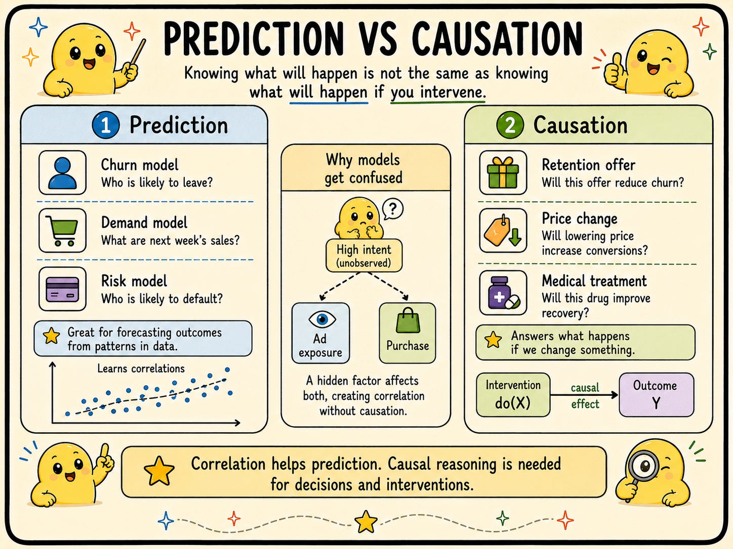
Most of the models we build as ML practitioners answer one question: What is likely to happen? A churn model predicts who will leave. A demand model predicts next week’s sales. A risk model predicts who will default.

But there is a second question that classical ML is surprisingly bad at answering: What will happen if I do something?

• Will this drug lower blood pressure?

• Will this retention campaign actually save customers?

• Will raising the minimum wage reduce employment?

• Will this new fraud check reduce losses without hurting conversion?

That second question is the domain of causal inference, and it is one of the most underrated skills in a data scientist’s toolkit.

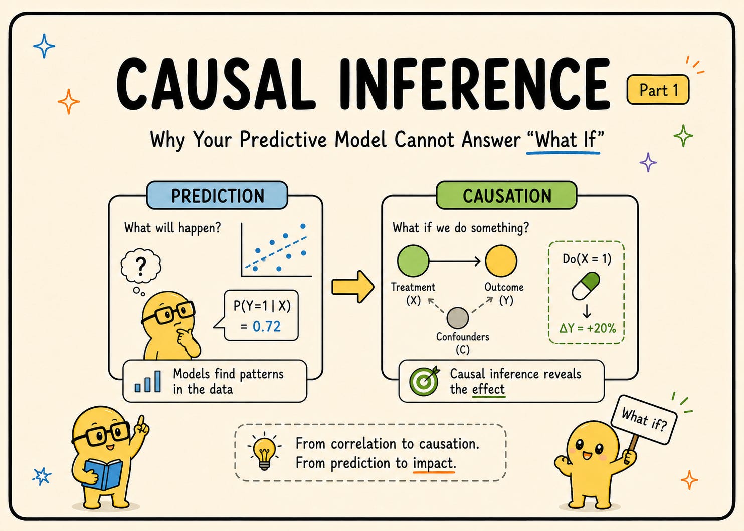
This is Part 1 of a three-part series:

• Part 1, this issue🆓: what causal inference is, why prediction is not causation, and the two theoretical frameworks that everything else builds on.

• Part 2: classical methodologies, from randomized experiments to quasi-experimental designs like Difference-in-Differences, Instrumental Variables, Regression Discontinuity, and Synthetic Control.

• Part 3: ML-based causal inference, including meta-learners, Double Machine Learning, causal forests, uplift modeling, and the tooling ecosystem.

A useful way to start is to separate two types of questions.

Predictive questions ask what is likely to happen.
Causal questions ask what will happen if we intervene and change something.

That sounds like a small distinction, but in practice it changes everything.

Consider three examples:

Patients who take a new medication recover faster than those who do not.
Does the drug work?

Maybe. But maybe doctors prescribe it more often to younger or healthier patients who would have recovered faster anyway. In that case, the drug is associated with better outcomes, but not necessarily causing them.

Users exposed to your retargeting ads purchase at 3x the rate of unexposed users.
Is the campaign working?

Not necessarily. Retargeting typically focuses on people who already visited your site or showed some intent. Those users were already more likely to buy. So a big part of that uplift may reflect who was targeted, not what the ad caused.

Students in smaller classes score higher on tests.
Do small classes improve learning?

Possibly. But wealthier districts may have smaller classes, better teachers, more support at home, and better infrastructure. Smaller classes may be correlated with better outcomes without being the full reason for them.

In all three cases, the data contains a real pattern, and a predictive model would happily learn it. In fact, it would probably learn it very well. That is the issue.

A predictive model is rewarded for finding patterns that improve accuracy. It does not care whether the pattern reflects a true causal effect or just a selection effect. If younger patients are more likely to receive a treatment and also more likely to recover, that helps prediction. If high-intent users are more likely to see ads and also more likely to purchase, that helps prediction too.

So predictive models often mix together:

• the effect of the action itself

• the effect of who received the action

• the effect of other hidden factors in the environment

This is where selection bias enters the picture. Treatment is rarely assigned at random. Doctors choose treatments. Ad platforms choose audiences. Schools choose class sizes. Humans and systems intervene in non-random ways all the time.

That means that observational data is not neutral. It reflects a world where treatment assignment is already entangled with other factors.

A quick test helps distinguish the two regimes:

• “Which patients are likely to be readmitted?” is prediction

• “Will this discharge protocol reduce readmissions?” is causation

• “Which customers are likely to churn?” is prediction

• “Whose churn will this retention offer actually prevent?” is causation

• “Which users are likely to convert?” is prediction

• “Will lowering the price increase conversions?” is causation

A good rule of thumb is this:

If the answer changes what you do, and your action changes the system, you are asking a causal question.

At the heart of causal inference is a very simple idea.

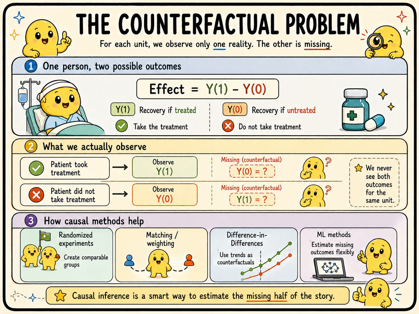
For a single unit, such as a patient, customer, city, or user, the causal effect of a treatment is:

effect(i) = Yᵢ(1) - Yᵢ(0)

Where:

• Yᵢ(1) is the outcome for unit i if treated

• Yᵢ(0) is the outcome for unit i if untreated

For example:

• recovery time if a patient takes a drug versus does not take it

• churn outcome if a customer receives an offer versus does not receive it

• spending if a user sees a promotion versus does not see it

The problem is that for any one unit, we only observe one of those outcomes.

If a patient takes the drug, we observe Y(1).
We do not observe Y(0) for that same patient.

If a customer gets the retention offer, we observe the world where they got it.
We never observe the parallel world where that same exact customer did not get it. That missing alternative outcome is called the counterfactual.

This is known as the fundamental problem of causal inference:
for each unit, we observe only one reality, and the other reality is missing.

This is why causal inference is often described as a missing data problem.

• We do not lack labels because of poor data collection.

• We lack them because they are fundamentally unobservable.
  You cannot simultaneously treat and not treat the same person at the same moment.

So every causal method is, in one way or another, a strategy for estimating that missing counterfactual as credibly as possible.

Here is the intuition behind some common approaches:

• Randomized experiments create treated and untreated groups that are statistically comparable, so one group can stand in for the missing counterfactual of the other.

• Matching and weighting try to construct comparison groups that look similar on observed covariates.

• Difference-in-Differences uses the trend of a control group as the counterfactual trend for the treated group.

• Synthetic control builds an artificial comparison unit by combining several untreated units.

• ML-based approaches estimate flexible response surfaces and heterogeneous treatment effects.

All of them are trying to answer the same question:

What would have happened to the treated units if they had not been treated?
Or, symmetrically,
What would have happened to untreated units if they had been treated?

That is the missing half of the story.

The notation above, with Y(1) and Y(0) for each unit, comes from the potential outcomes framework, often associated with Donald Rubin.

This framework is powerful because it gives precise definitions for the quantities we care about.

This is the average effect of treatment across the whole population.

Example:
What is the average effect of a new medication on recovery time across all eligible patients?

This is the effect among the units that actually received treatment.

Example:
Did the ad campaign work for the users who actually saw the ad?

This is often highly relevant in business, because companies frequently want to understand whether an action delivered value for the people it was applied to.

This is the treatment effect for a subgroup defined by features X.

Example:

• Does this therapy work better for patients over 65?

• Do price reductions work better for new users than returning users?

• Which customers are most likely to respond positively to a retention offer?

This is the quantity behind personalization, uplift modeling, and much of modern ML-based causal inference.

To identify causal effects from observational data, we usually rely on a few key assumptions.

Conditional on observed covariates X, treatment assignment is as good as random.

In plain English: once you account for the variables you observed, there are no hidden confounders left.

This is a very strong assumption, and often the least testable one.

If an important factor is missing, such as severity of illness, purchase intent, or motivation, the estimate can still be biased.

Every type of unit must have some chance of receiving each treatment.

If one subgroup never receives treatment, you cannot estimate the treatment effect for that subgroup because there is no counterfactual support in the data.

A simple way to say it is: no overlap, no comparison, no causal estimate

This stands for the Stable Unit Treatment Value Assumption.

It usually includes two ideas:

• no interference between units

• a well-defined treatment

No interference means that my treatment should not directly change your outcome. That can fail in many real settings, such as epidemics, social networks, marketplaces, or recommender systems.

A well-defined treatment means the intervention should be clearly specified. “Received a marketing campaign” may sound simple, but was it the same creative, the same frequency, the same channel, and the same timing for everyone? If not, the treatment may actually be multiple treatments blended together.

These assumptions are where much of the real work lies. In practice, causal inference is often less about fancy estimators and more about whether your assumptions are believable.

The second major framework is associated with Judea Pearl and Structural Causal Models, often represented with Directed Acyclic Graphs, or DAGs.

Why are DAGs useful? Because they force you to make your assumptions explicit.

Instead of vaguely saying “we controlled for relevant variables,” a DAG makes you specify:

• what causes what

• which paths create bias

• which variables should be adjusted for

• which variables should not be adjusted for

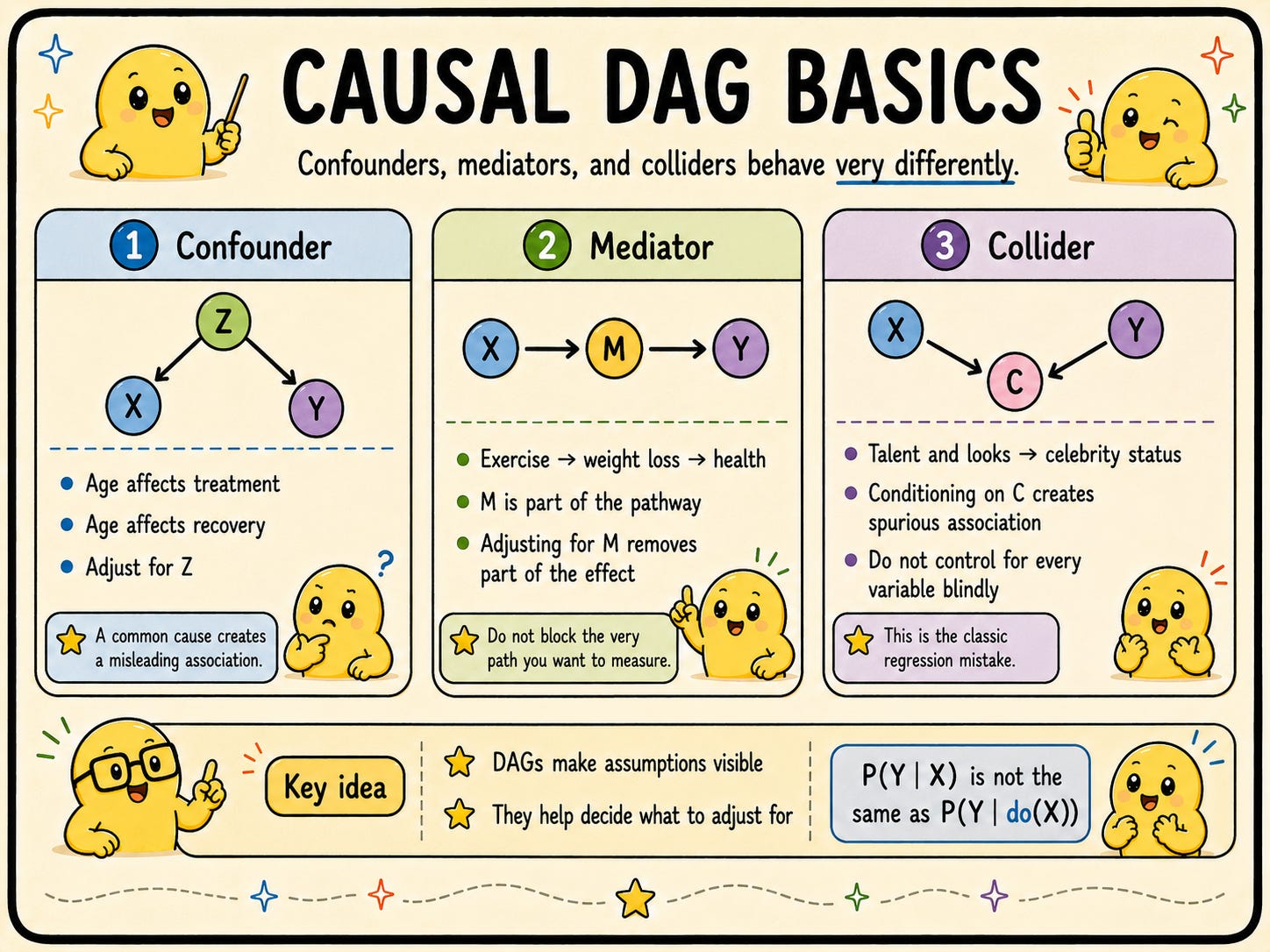
Three patterns are especially important:

A confounder is a common cause of both treatment and outcome.

Example:
Age affects both whether a patient receives a treatment and how likely they are to recover.

In graph form:

Treatment ← Age → Outcome

If you fail to adjust for age, you may attribute to the treatment what is actually due to age.

A mediator lies on the causal path from treatment to outcome.

Example:
Exercise improves health partly through weight loss.

In graph form:

Exercise → Weight loss → Health

If your goal is to estimate the total effect of exercise on health, adjusting for weight loss would remove part of the effect you actually want to measure.

A collider is a common effect of two variables.

Example:
Suppose both talent and looks influence whether someone becomes a celebrity.

In graph form:

Talent → Celebrity ← Looks

If you condition on celebrity status, talent and looks can become spuriously associated in your selected sample, even if they were independent in the full population.

This is one of the biggest conceptual traps in applied work.

It explains why “just control for everything” is not a safe strategy.
Controlling for the wrong variable can create bias rather than remove it.

One of Pearl’s most useful ideas is the distinction between:

• P(Y | X), what happens when we observe X

• P(Y | do(X)), what happens when we intervene and set X

These are not the same thing.

A classic example is that people who carry lighters may have higher lung cancer rates. But confiscating lighters would not reduce lung cancer. The lighter is associated with smoking, which is the real cause.

So:

• observing lighter ownership tells us something about risk

• intervening on lighter ownership does not produce the same effect

That is the gap between correlation and causation in one line of notation.

You do not need to master the graphical rules on day one, but getting comfortable with DAG thinking is one of the highest-leverage habits in causal work.

In real projects, the two frameworks are complementary.

A simple way to think about it is:

• DAGs help you reason about the data-generating process

• Potential outcomes help you define the target estimand and the statistical problem

In practice:

• use DAGs to think through confounders, mediators, colliders, and identifiability

• use potential outcomes to define whether you want ATE, ATT, or CATE, and then choose an appropriate estimator

A very good habit, one that takes only a few minutes, is this:

Before running any causal analysis, draw the DAG on paper. Even a rough sketch helps. It forces you to state your assumptions before the data starts tempting you into convenient stories. That small discipline can save you from many bad analyses.

Causal inference matters because many real business and product questions are intervention questions disguised as analytics questions.

Examples:

• Should we send this offer?

• Should we lower the price?

• Should we change the onboarding flow?

• Should we add a fraud rule?

• Should we contact this customer?

• Should we recommend this treatment?

A predictive model can tell you who is likely to do something.
A causal approach helps you estimate what your action will change.

That is the difference between forecasting the system and acting on the system.

Both are useful.
They are just not the same.

Now that we know what we are estimating, and under which assumptions, the next step is methodology.

In Part 2, we will move from theory to practice and cover the main classical tools for estimating causal effects:

• randomized experiments

• matching

• Difference-in-Differences

• Instrumental Variables

• Regression Discontinuity

• Synthetic Control

These are the workhorse methods you reach for when you need causal answers and a clean randomized experiment is impossible, unethical, or simply too slow.

If Part 1 was about learning to ask the right question, Part 2 is about learning how to answer it.