
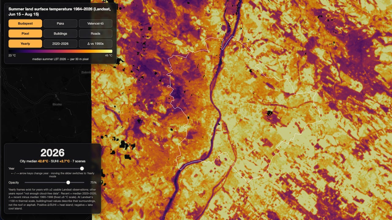
We will build one map: the typical (median) land surface temperature (LST) of a Hungarian study area in summer 2026, from free Landsat satellite data. Every step shows its work — you will see the raw data, every filter, and every intermediate result before the final map.
For the interactive version, click here
For the YT version, click
What is LST? The temperature of the surface itself — asphalt, rooftops, treetops, water — not the air temperature from a weather report. A parking lot can be 20 °C hotter than the air above it. That is why LST is the standard tool for studying urban heat islands.
Two honest caveats. Landsat passes over Hungary mid-morning, so we map morning heat (afternoon is hotter). And it cannot see through clouds, so the map is built only from clear moments. Neither changes where the hot and cool spots are.
The workflow:
Tools
Choose a study area → fetch and check its boundary → frame a bounding box
Search the satellite catalog → look at what we found before downloading
Download one scene and inspect the raw numbers
Convert to °C and remove clouds, filter by filter
Put the scene on Hungary’s map grid
Repeat for every scene (a plain loop — same code you already saw)
Median composite → the final map
Bonus: hang the same heat on buildings and roads
No accounts, no API keys — just Python and an internet connection.
import warnings
import geopandas as gpd
import matplotlib as mpl
import matplotlib.pyplot as plt
import numpy as np
import osmnx as ox
import planetary_computer
import pystac_client
import rioxarray
from rasterio.enums import Resampling
from rasterio.warp import transform_bounds
from shapely.geometry import box, shape
import os
os.environ["GDAL_DISABLE_READDIR_ON_OPEN"] = "EMPTY_DIR"  # faster remote reads
ox.settings.use_cache = False                             # no cache folder here
# If the main OpenStreetMap query server is busy (easy to hit in a classroom
# where everyone shares one network), switch to a public mirror:
# ox.settings.overpass_url = "https://maps.mail.ru/osm/tools/overpass/api"
# ox.settings.overpass_rate_limit = False
warnings.filterwarnings("ignore")                          # keep the output clean
print("geopandas", gpd.__version__, "| osmnx", ox.__version__,
      "| rioxarray", rioxarray.__version__)
Output:
geopandas 1.1.2 | osmnx 2.0.7 | rioxarray 0.21.0
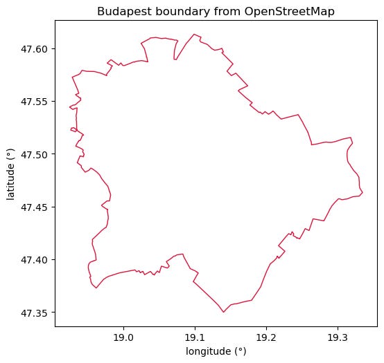
One variable picks the area. We verify the boundary before trusting it: it must be a polygon (not a point!) with roughly the right area — a wrong geocoder match would fail loudly here, which is exactly what we want.
CITY = "budapest"     # <-- change me: "budapest", "paks", or "velence"
YEAR = 2026
CITIES = {
    "budapest": {"query": "Budapest, Hungary", "expected_km2": 525},
    "paks":     {"query": "Paks, Hungary",     "expected_km2": 154},
    "velence":  {"query": "Velencei-tó",       "expected_km2": 14},
}
query = CITIES[CITY]["query"]
expected = CITIES[CITY]["expected_km2"]
place = query.split(",")[0]
boundary = ox.geocode_to_gdf(query)          # the boundary, from OpenStreetMap
EOV = "EPSG:23700"                           # Hungary's national grid (metres)
boundary_eov = boundary.to_crs(EOV)
area_km2 = boundary_eov.geometry.iloc[0].area / 1e6
print("geometry type:", boundary.geometry.iloc[0].geom_type)
print(f"area: {area_km2:.0f} km²  (expected ~{expected} km²)")
assert boundary.geometry.iloc[0].geom_type in ("Polygon", "MultiPolygon")
assert 0.7 * expected < area_km2 < 1.4 * expected, "wrong geocoder match?"
print("boundary check passed ✔")
Output:
geometry type: Polygon
area: 526 km²  (expected ~525 km²)
boundary check passed ✔
# first look: the boundary itself, axes in degrees (EPSG:4326)
ax = boundary.plot(figsize=(6, 6), facecolor="none", edgecolor="crimson")
ax.set_title(f"{place} boundary from OpenStreetMap")
ax.set_xlabel("longitude (°)"); ax.set_ylabel("latitude (°)")
plt.show()
# frame a padded bounding box around the boundary - our download window
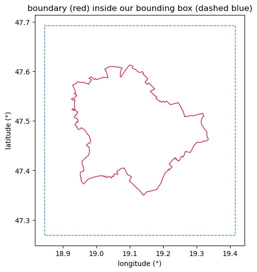
PAD = 0.08  # degrees ≈ 6-9 km
w, s, e, n = boundary.total_bounds
BBOX = (w - PAD, s - PAD, e + PAD, n + PAD)
ax = boundary.plot(figsize=(6, 6), facecolor="none", edgecolor="crimson")
gpd.GeoSeries([box(*BBOX)], crs="EPSG:4326").plot(
    ax=ax, facecolor="none", edgecolor="steelblue", linestyle="--")
ax.set_title("boundary (red) inside our bounding box (dashed blue)")
ax.set_xlabel("longitude (°)"); ax.set_ylabel("latitude (°)")
plt.show()
print("BBOX (west, south, east, north):", tuple(round(v, 3) for v in BBOX))
Output:
BBOX (west, south, east, north): (np.float64(18.845), np.float64(47.27), np.float64(19.415), np.float64(47.693))
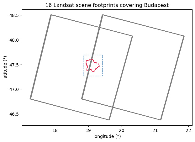
The Microsoft Planetary Computer hosts the full Landsat archive behind a free STAC catalog. We ask for every scene touching our box between June 15 and August 15, keep the quality tier (”T1”), and — before downloading a single pixel — draw the scene footprints to see what we are dealing with.
catalog = pystac_client.Client.open(
    "https://planetarycomputer.microsoft.com/api/stac/v1",
    modifier=planetary_computer.sign_inplace,   # signs download links, no account
)
search = catalog.search(collections=["landsat-c2-l2"], bbox=list(BBOX),
                        datetime=f"{YEAR}-06-15/{YEAR}-08-15")
items = [it for it in search.items()
         if it.properties["landsat:collection_category"] == "T1"]
items.sort(key=lambda it: it.datetime)
print(f"{len(items)} Tier-1 scenes, summer {YEAR}:")
for it in items:
    p = it.properties
    print(f"  {it.datetime:%Y-%m-%d}  {p['platform']:>9}"
          f"  {p['eo:cloud_cover']:5.1f}% cloud")
assert len(items) >= 3, "need a few scenes for a meaningful median"
Output:
16 Tier-1 scenes, summer 2026:
  2026-06-16  landsat-9    5.2% cloud
  2026-06-17  landsat-8   39.5% cloud
  2026-06-24  landsat-8    7.6% cloud
  2026-06-25  landsat-9    0.3% cloud
  2026-07-02  landsat-9   50.4% cloud
  2026-07-03  landsat-8   32.0% cloud
  2026-07-10  landsat-8   39.6% cloud
... (9 more lines)
# the data-collection map: every scene footprint over our area
footprints = gpd.GeoDataFrame(
    {"date": [f"{it.datetime:%m-%d}" for it in items]},
    geometry=[shape(it.geometry) for it in items], crs="EPSG:4326")
ax = footprints.plot(figsize=(7, 7), facecolor="none", edgecolor="grey")
gpd.GeoSeries([box(*BBOX)], crs="EPSG:4326").plot(
    ax=ax, facecolor="none", edgecolor="steelblue", linestyle="--")
boundary.plot(ax=ax, facecolor="none", edgecolor="crimson")
ax.set_title(f"{len(items)} Landsat scene footprints covering {place}")
ax.set_xlabel("longitude (°)"); ax.set_ylabel("latitude (°)")
plt.show()
# keep the ~10 clearest scenes so the tutorial downloads stay small
items = sorted(items, key=lambda it: it.properties["eo:cloud_cover"])[:10]
items.sort(key=lambda it: it.datetime)
print(f"keeping the {len(items)} clearest scenes for this tutorial "
      "(the full pipeline uses all of them)")
Output:
keeping the 10 clearest scenes for this tutorial (the full pipeline uses all of them)
We download only our bounding-box window (a full scene would be ~1 GB for all bands; our windows are a few MB). Four bands per scene:
bandasset keymeaningST_B10lwir11surface temperature, as raw digital numbersQA_PIXELqa_pixelcloud / shadow / snow flags, bit by bitQA_RADSATqa_radsatsensor saturation flagsST_QAqahow uncertain the temperature is (×0.01 K)
item = items[0]
print("scene:", item.id)
# open lazily, crop to our box (in the scene's own CRS), then download
st = rioxarray.open_rasterio(item.assets["lwir11"].href)
window = transform_bounds("EPSG:4326", st.rio.crs, *BBOX)
st = st.rio.clip_box(*window).squeeze("band", drop=True).load()
print("scene CRS:      ", st.rio.crs, "(a UTM zone - metres)")
print("window size:    ", st.shape, f"= {st.size/1e6:.1f} M pixels")
print("raw value range:", int(st.min()), "to", int(st.max()), " <- NOT degrees!")
Output:
scene: LC09_L2SP_188027_20260616_02_T1
scene CRS:       EPSG:32634 (a UTM zone - metres)
window size:     (1604, 1470) = 2.4 M pixels
raw value range: 0 to 51706  <- NOT degrees!
# look at the raw digital numbers - recognisable, but meaningless units
fig, (ax1, ax2) = plt.subplots(1, 2, figsize=(12, 4.5))
st.plot.imshow(ax=ax1, cmap="Greys_r", add_colorbar=True)
ax1.set_title("raw digital numbers (DN)"); ax1.set_aspect("equal")
ax2.hist(st.values.ravel(), bins=100, color="grey")
ax2.set_title("DN histogram - note the spike at 0 = nodata")
ax2.set_xlabel("DN"); ax2.set_ylabel("pixel count")
plt.tight_layout(); plt.show()
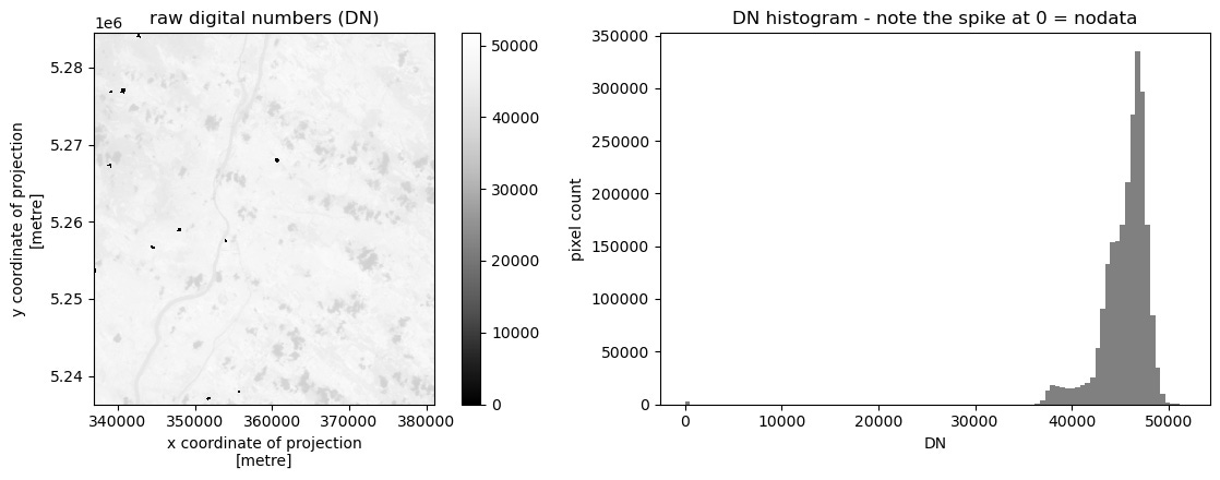
# USGS gives the official conversion: DN -> Kelvin -> °C
lst = st.astype("float32") * 0.00341802 + 149.0 - 273.15
lst = lst.where(st != 0)   # DN 0 means "no data", not "cold"
print(f"°C range: {float(lst.min()):.1f} to {float(lst.max()):.1f}")
print("plausible for a Hungarian summer morning? (expect roughly 15-55 °C)")
ax = lst.plot.imshow(figsize=(7, 5.5), cmap="inferno", add_colorbar=True)
plt.gca().set_title("the same scene in °C - but clouds are still in there!")
plt.gca().set_aspect("equal"); plt.show()
Output:
°C range: 0.7 to 52.6
plausible for a Hungarian summer morning? (expect roughly 15-55 °C)
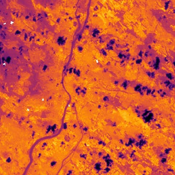
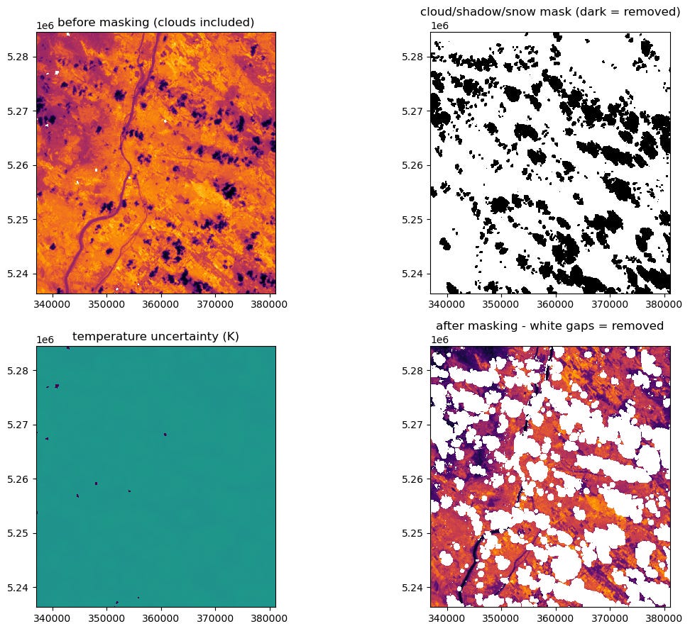
Clouds are cold, so unmasked clouds would poison a heat map with fake cold patches. Landsat ships quality bands for exactly this. We apply each filter separately first, so you can see what each one removes — then combine them.
qa_pixel = rioxarray.open_rasterio(item.assets["qa_pixel"].href
    ).rio.clip_box(*window).squeeze("band", drop=True).load()
qa_radsat = rioxarray.open_rasterio(item.assets["qa_radsat"].href
    ).rio.clip_box(*window).squeeze("band", drop=True).load()
st_qa = rioxarray.open_rasterio(item.assets["qa"].href
    ).rio.clip_box(*window).squeeze("band", drop=True).load()
BAD_BITS = 0b00111111   # bits 0-5: fill, dilated cloud, cirrus, cloud, shadow, snow
MAX_UNC_K = 4.0         # drop pixels whose temperature error exceeds this
mask_cloud = (qa_pixel & BAD_BITS) != 0     # any cloud-ish bit set
mask_sat   = qa_radsat != 0                 # sensor saturated
mask_unc   = (st_qa * 0.01) > MAX_UNC_K     # uncertain temperature
for name, m in [("cloud/shadow/snow bits", mask_cloud),
                ("saturation", mask_sat),
                (f"uncertainty > {MAX_UNC_K:.0f} K", mask_unc)]:
    print(f"{name:24s} removes {float(m.mean()):5.1%} of pixels")
Output:
cloud/shadow/snow bits   removes 25.2% of pixels
saturation               removes  0.0% of pixels
uncertainty > 4 K        removes 39.2% of pixels
lst_clean = lst.where(~mask_cloud & ~mask_sat & ~mask_unc)
print(f"pixels kept: {float(lst_clean.notnull().mean()):.1%}")
fig, axes = plt.subplots(2, 2, figsize=(12, 9))
lst.plot.imshow(ax=axes[0, 0], cmap="inferno", add_colorbar=False)
axes[0, 0].set_title("before masking (clouds included)")
mask_cloud.plot.imshow(ax=axes[0, 1], cmap="Greys", add_colorbar=False)
axes[0, 1].set_title("cloud/shadow/snow mask (dark = removed)")
(st_qa * 0.01).plot.imshow(ax=axes[1, 0], cmap="viridis", add_colorbar=False)
axes[1, 0].set_title("temperature uncertainty (K)")
lst_clean.plot.imshow(ax=axes[1, 1], cmap="inferno", add_colorbar=False)
axes[1, 1].set_title("after masking - white gaps = removed")
for ax in axes.ravel():
    ax.set_aspect("equal"); ax.set_xlabel(""); ax.set_ylabel("")
plt.tight_layout(); plt.show()
Output:
pixels kept: 57.2%
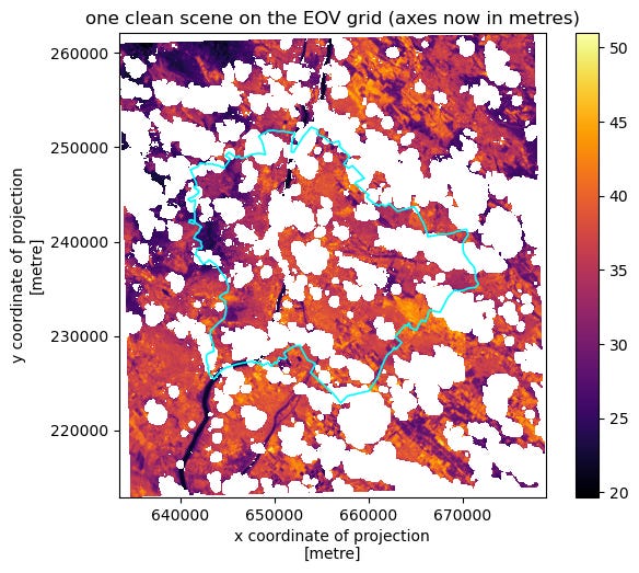
Different scenes come in different UTM zones. To combine them we need ONE shared grid: EPSG:23700 (the Hungarian EOV grid), 30 m pixels. We check the pixel size afterwards — a classic silent-error spot in map work.
lst_clean.rio.write_nodata(np.nan, inplace=True)
template = lst_clean.rio.reproject(EOV, resolution=30,
                                   resampling=Resampling.bilinear, nodata=np.nan)
px_x = float(template.x[1] - template.x[0])
px_y = float(template.y[0] - template.y[1])
print("new CRS:", template.rio.crs)
print(f"pixel size: {px_x:.0f} m x {px_y:.0f} m -> area {px_x*px_y:.0f} m²"
      "  (must be 900)")
assert abs(px_x * px_y - 900) < 1, "pixel size wrong after reprojection!"
ax = template.plot.imshow(figsize=(7, 5.5), cmap="inferno", add_colorbar=True)
boundary_eov.boundary.plot(ax=plt.gca(), color="cyan", linewidth=1.2)
plt.gca().set_title("one clean scene on the EOV grid (axes now in metres)")
plt.gca().set_aspect("equal"); plt.show()
Output:
new CRS: EPSG:23700
pixel size: 30 m x 30 m -> area 900 m²  (must be 900)
Exactly the lines you have already seen, repeated per scene — download, convert, mask, reproject. Each scene is aligned onto the grid of the first one (reproject_match), so every pixel means the same place in every scene.
scenes = [template]                    # the scene we already processed
for item in items[1:]:
    st = rioxarray.open_rasterio(item.assets["lwir11"].href)
    window = transform_bounds("EPSG:4326", st.rio.crs, *BBOX)
    st = st.rio.clip_box(*window).squeeze("band", drop=True).load()
    qa_pixel = rioxarray.open_rasterio(item.assets["qa_pixel"].href
        ).rio.clip_box(*window).squeeze("band", drop=True).load()
    qa_radsat = rioxarray.open_rasterio(item.assets["qa_radsat"].href
        ).rio.clip_box(*window).squeeze("band", drop=True).load()
    st_qa = rioxarray.open_rasterio(item.assets["qa"].href
        ).rio.clip_box(*window).squeeze("band", drop=True).load()
    lst = (st.astype("float32") * 0.00341802 + 149.0 - 273.15).where(st != 0)
    lst = lst.where(((qa_pixel & BAD_BITS) == 0) & (qa_radsat == 0)
                    & ((st_qa * 0.01) <= MAX_UNC_K))
    lst.rio.write_nodata(np.nan, inplace=True)
    aligned = lst.rio.reproject_match(template, resampling=Resampling.bilinear)
    scenes.append(aligned)
    print(f"{item.datetime:%Y-%m-%d}  usable {float(aligned.notnull().mean()):5.1%}"
          f"  {item.properties['platform']}")
print(f"\n{len(scenes)} scenes, all on the same grid:",
      len({s.shape for s in scenes}) == 1)
Output:
2026-06-24  usable 62.5%  landsat-8
2026-06-25  usable 61.0%  landsat-9
2026-07-03  usable  2.6%  landsat-8
2026-07-18  usable 60.4%  landsat-9
2026-07-26  usable 41.2%  landsat-8
2026-08-03  usable 90.2%  landsat-9
2026-08-04  usable 58.6%  landsat-8
2026-08-11  usable 16.0%  landsat-8
... (2 more lines)
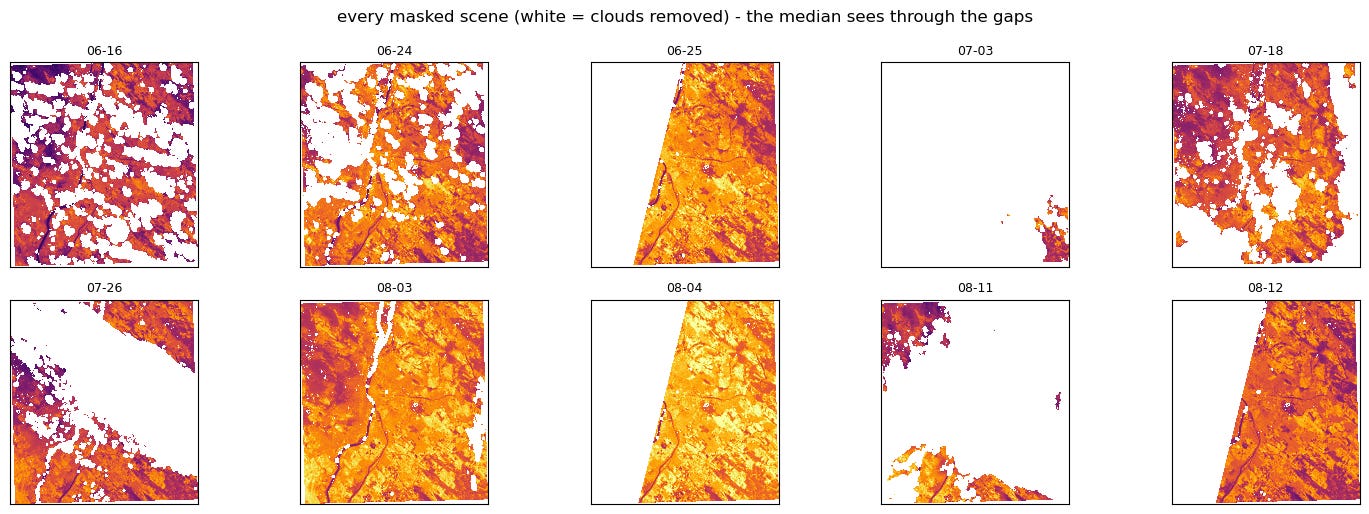
# see everything that goes into the median - one thumbnail per scene
cols = 5
rows = int(np.ceil(len(scenes) / cols))
fig, axes = plt.subplots(rows, cols, figsize=(3 * cols, 2.6 * rows))
for ax, s, it in zip(np.ravel(axes), scenes, items):
    s.plot.imshow(ax=ax, cmap="inferno", vmin=15, vmax=55, add_colorbar=False)
    ax.set_title(f"{it.datetime:%m-%d}", fontsize=9)
for ax in np.ravel(axes):
    ax.set_aspect("equal"); ax.set_xticks([]); ax.set_yticks([])
    ax.set_xlabel(""); ax.set_ylabel("")
plt.suptitle("every masked scene (white = clouds removed) - the median sees through the gaps")
plt.tight_layout(); plt.show()
Step 8 — The median composite: the final map
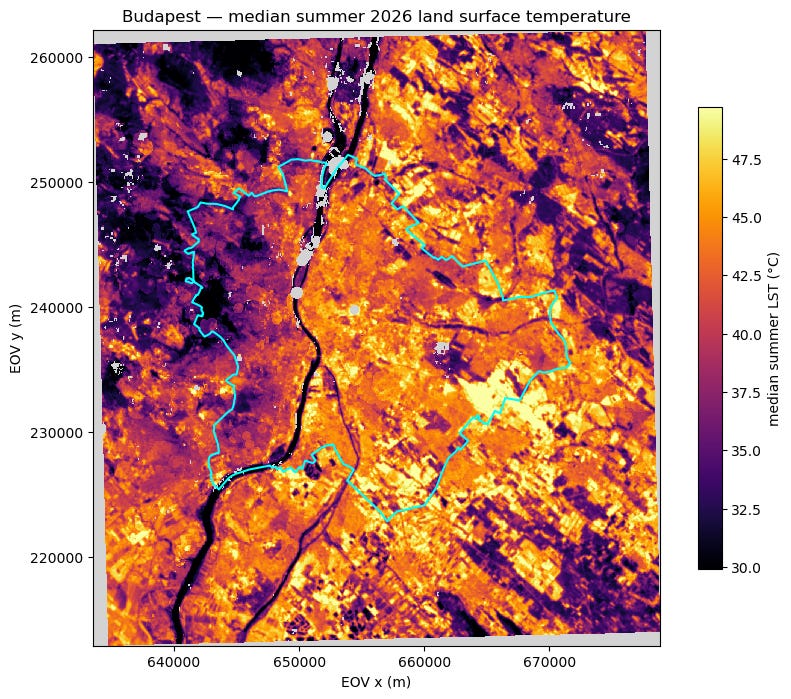
Per pixel, the median of all clear looks. Clouds moved between dates, so where one scene has a hole another usually has data — the median heals the gaps with real measurements and ignores leftover outliers.
from scipy import ndimage
stack  = np.stack([s.values for s in scenes])
median = np.nanmedian(stack, axis=0)
n_obs  = np.sum(~np.isnan(stack), axis=0)
print(f"stack shape (scenes, rows, cols): {stack.shape}")
print(f"pixels with ≥1 clear look: {(n_obs > 0).mean():.1%}")
print(f"median °C range: {np.nanmin(median):.1f} to {np.nanmax(median):.1f}")
# --- close the leftover holes -------------------------------------------
# A grey pixel is a place where EVERY scene was cloudy. We fill it from its
# neighbours: each pass gives an empty pixel the average of the filled pixels
# touching it, so the fill grows inward from the rim of each hole, one 30 m
# ring at a time. MAX_PASSES caps how far it may grow (60 passes ≈ 1.8 km),
# so small cloud holes close but genuinely unobserved regions stay grey.
MAX_PASSES = 60
filled      = median.astype("float64").copy()
filled_mask = np.zeros(filled.shape, dtype=bool)   # True = invented, not measured
for _ in range(MAX_PASSES):
    known = np.isfinite(filled)
    holes = ~known
    if not holes.any():
        break
    neigh_sum = ndimage.uniform_filter(np.where(known, filled, 0.0), size=3) * 9
    neigh_cnt = ndimage.uniform_filter(known.astype(float), size=3) * 9
    ready = holes & (neigh_cnt > 0.5)              # holes touching known data
    if not ready.any():
        break                                       # nothing left we can reach
    filled[ready] = neigh_sum[ready] / neigh_cnt[ready]
    filled_mask[ready] = True
print(f"filled {filled_mask.sum():,} px by interpolation "
      f"({filled_mask.mean():.1%} of the map); "
      f"{np.isnan(filled).sum():,} px still unobserved")
# --- draw it -------------------------------------------------------------
lst_map = template.copy(data=filled)
vmin, vmax = np.nanpercentile(filled, [2, 98])
cmap = mpl.colormaps["inferno"].copy(); cmap.set_bad("lightgrey")
fig, ax = plt.subplots(figsize=(10, 8))
im = lst_map.plot.imshow(ax=ax, cmap=cmap, vmin=vmin, vmax=vmax, add_colorbar=False)
boundary_eov.boundary.plot(ax=ax, color="cyan", linewidth=1.5)
fig.colorbar(im, ax=ax, shrink=0.75, label="median summer LST (°C)")
# zoom to the area of interest - the ragged corners outside are just the
# edge of the satellite swath, not missing measurements
pad = 5000
minx, miny, maxx, maxy = boundary_eov.total_bounds
ax.set_xlim(minx - pad, maxx + pad); ax.set_ylim(miny - pad, maxy + pad)
ax.set_title(f"{place} — median summer {YEAR} land surface temperature "
             f"({filled_mask.mean():.0%} gap-filled)")
ax.set_xlabel("EOV x (m)"); ax.set_ylabel("EOV y (m)"); ax.set_aspect("equal")
plt.show()
Output:
stack shape (scenes, rows, cols): (10, 1641, 1511)
pixels with ≥1 clear look: 94.1%
median °C range: 20.8 to 61.6
# quality companion: how many clear looks stand behind each pixel?
fig, ax = plt.subplots(figsize=(8, 6))
im = template.copy(data=n_obs.astype(float)).plot.imshow(
    ax=ax, cmap="viridis", add_colorbar=False)
boundary_eov.boundary.plot(ax=ax, color="white", linewidth=1.2)
fig.colorbar(im, ax=ax, shrink=0.75, label=f"clear looks (of {len(scenes)} scenes)")
ax.set_title("trust map: more looks = more reliable median")
ax.set_xlabel("EOV x (m)"); ax.set_ylabel("EOV y (m)"); ax.set_aspect("equal")
plt.show()
Three canvases for one dataset: pixels show the measurement, buildings show exposure (where people live), roads show the sealed network that drives the heat. Honesty rule: a thermal pixel is a ~100 m mixture, so a small building’s or street’s value describes its surroundings, not its own roof or asphalt. We fetch OSM only for a small circle so this stays fast.
centre = boundary_eov.geometry.iloc[0].representative_point()
demo = gpd.GeoSeries([centre.buffer(2500)], crs=EOV).to_crs("EPSG:4326").iloc[0]
bldg = ox.features_from_polygon(demo, {"building": True})
bldg = bldg[bldg.geometry.geom_type.isin(["Polygon", "MultiPolygon"])].to_crs(EOV)
road = ox.features_from_polygon(
    demo, {"highway": ["primary", "secondary", "tertiary", "residential"]})
road = road[road.geometry.geom_type.isin(["LineString", "MultiLineString"])].to_crs(EOV)
print(f"{len(bldg)} buildings, {len(road)} road ways in the demo circle")
# temperature of the pixel under each building / road midpoint (nearest pixel)
bldg["lst"] = [float(lst_map.sel(x=p.x, y=p.y, method="nearest"))
               for p in bldg.geometry.representative_point()]
road["lst"] = [float(lst_map.sel(x=p.x, y=p.y, method="nearest"))
               for p in road.geometry.interpolate(0.5, normalized=True)]
road["geometry"] = road.geometry.buffer(6)   # 6 m half-width, for drawing
minx, miny, maxx, maxy = centre.buffer(2500).bounds
fig, axes = plt.subplots(1, 3, figsize=(15, 5.5))
lst_map.plot.imshow(ax=axes[0], cmap=cmap, vmin=vmin, vmax=vmax, add_colorbar=False)
axes[0].set_title("pixels — the measurement")
bldg.plot(ax=axes[1], column="lst", cmap=cmap, vmin=vmin, vmax=vmax, linewidth=0)
axes[1].set_title("buildings — where people live")
road.plot(ax=axes[2], column="lst", cmap=cmap, vmin=vmin, vmax=vmax, linewidth=0)
axes[2].set_title("roads — the sealed network")
for ax in axes:
    ax.set_xlim(minx, maxx); ax.set_ylim(miny, maxy)
    ax.set_aspect("equal"); ax.set_xticks([]); ax.set_yticks([])
    ax.set_facecolor("#111114"); ax.set_xlabel(""); ax.set_ylabel("")
sm = plt.cm.ScalarMappable(cmap=cmap, norm=plt.Normalize(vmin, vmax))
fig.colorbar(sm, ax=axes, shrink=0.8, label="median summer LST (°C)")
fig.suptitle(f"{place}: one heat field, three maps (demo circle, r = 2.5 km)")
plt.show()
Another area: set
CITY = "paks"or"velence"in Step 2, rerun all. Paks has a nuclear power plant by the cool Danube; Lake Velence flips the story into a cool island.Another year: change
YEAR(Landsat 8 starts 2013). Fewer or cloudier scenes → watch the trust map change.Your own city: add it to
CITIES(a geocodable name + rough area). Outside Hungary also changeEOVto a metric CRS that fits (e.g."EPSG:32633"for Vienna).Who eats the pixels? Set
MAX_UNC_K = 3.0in Step 5 and rerun (both Step 5 and the Step 7 loop use it) — watch how much data one number costs.
Data: Landsat Collection 2 Level-2 (USGS/NASA) via Microsoft Planetary Computer. Boundaries, buildings, roads © OpenStreetMap contributors. Made for the “New Science of Maps” YouTube series.
No posts
Comments
Nothing yet. Say the first thing.
Sign in to join the conversation.