Not Quite So Cosmic Influenza (part 9)

So… we’ve got a Mann-Whitney U-test and a Generalised Linear Model indicating that high levels of unseasonably warm winter days are associated with lower levels of influenza mortality for England & Wales over the period 1920 – 2022. This might sound groovy but it makes me uneasy, and it makes me uneasy because I’m using statistical techniques developed for cross-sectional datasets and not time series data.

Yes indeed, I’ve got nice-looking and rather interesting results on the table, but these can easily be misleading. I’ve already mentioned a potential confounding factor of warmer winters tending to be recent winters, and earlier in this series we saw mortality for influenza in sharp decline over the years. Put the two together and you’ve got bias bigger than my brunch today, and it sure was a big brunch!

Time series modelling needs to come to the rescue, and that means I’ll be reaching for my ARIMA spanner once again. If I get another positive result supporting the hot winter = less flu death hypothesis it means cake and champagne all round. If not, then it is a lesson learned, and I’m hoping some readers will start asking searching questions of researchers who fail to see the pitfalls of using fancy cross-sectional methods on time series data – and epidemiologists are amongst the worst offenders1.

You know what’s coming next.

Yep, here it comes…

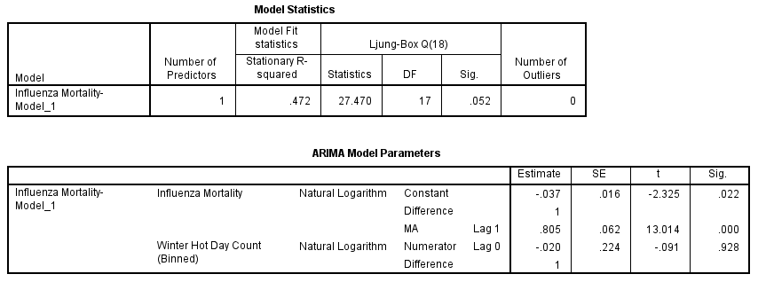
This is some of the output for an ARIMA(0,1,1) model that attempts to track influenza mortality (deaths/100k) across England & Wales over the period 1920 – 2022. It’s a modest-fitting model, with a stationary R-square of just 0.472, but this sort of figure is pretty much bang in the middle of the ballpark for tracking something as complex as death over time. No worries there.

Where we should worry is that I’ve forced the binary indicator for high and low levels of unseasonably warm winter days (that we saw dancing around in part 8 in a most convincing manner) into the model as an independent predictor variable. This time it has stubbed its toe and come a cropper with a p-value of p=0.928, meaning it is pretty useless as a time-dependent indicator for mortality.

Computer says no, and just to rub it in I’ll reveal the cross-correlation function plot for the winter hot day count (raw counts) with influenza mortality:

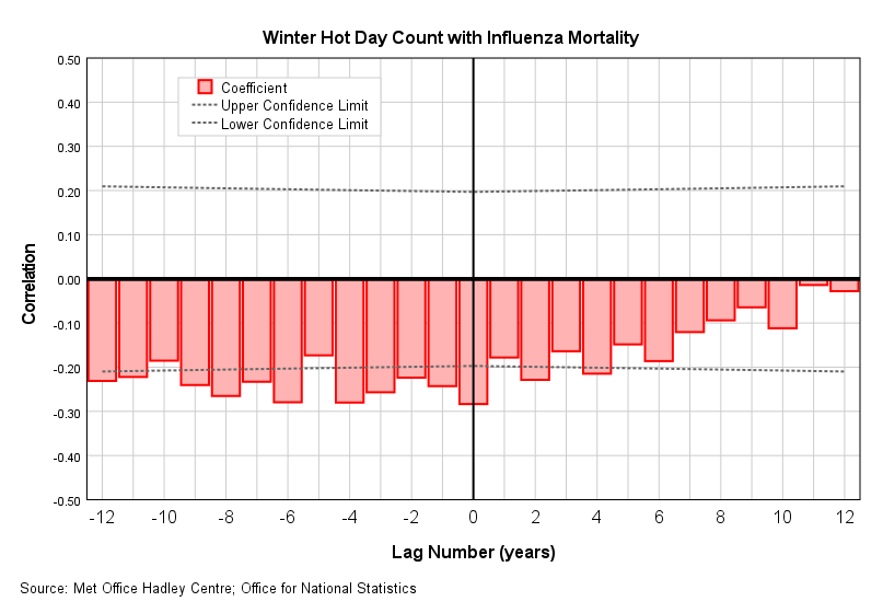
Please note the sign of the lags associated with that palisade of negative-going bars. Aside from one bar at lag zero (i.e. same year) they are all negative, which means the cart has been put before the horse. By that I mean the relationship between the winter unseasonably hot day count and influenza mortality is the wrong way round, in that mortality is declining before the winter warm day count rises.

Here’s the thing…

The rather popular classical methods of statistical analysis like Mann-Whitney U, ANOVA, MANOVA, linear regression, non-linear regression, bivariate correlation, partial correlation, independent samples t-test, paired samples t-test, Kruskal-Wallis 1-way, Kolmogorov-Smirnov, Jonckheere-Terpstra, Moses extreme reaction, McNemar, Cochran’s Q, Wilcoxon matched pair, Friedman’s 2-way, logistic regression, loglinear analysis, partial least squares regression, 2-stage least squares regression, multinomial logistic regression, and Generalised Linear Modelling do not care one jot about the arrow of time within the dataset, which is why they can show a result that is utterly meaningless in the real world. The same goes for those fashionable Bayes variants of the same classical methods. A good many researchers gloss over this brutal fact in their race to publish; yet death, disease, illness, recovery, treatment and, indeed, pretty much every aspect of human health are quintessentially time-dependent vectors.

So… here I am blowing the whistle on my own work so you can see how the dastardly tricks of the sleeve may easily slip by. Flipping back to our consideration of the above plot we can see there’s a sensibly placed negative-going bar at lag zero, and a weeny pip-squeak of a bar at a lag of +2 years but these are pretty small potatoes in the scheme of things (and somebody would need to explain away a 2-year delay). I suggest we clear our throats, gargle with gin, ignore these results and simmer down.

Yet another Dee hypothesis bites the dust, but the joy remains in the baking.

Not a lark, but a switched-on and groovy reader who mentioned CHANGE in temperature as a possible driver of influenza. Now this sort of thing gets me reaching for a clean apron and my big cooking pot.

I can’t go granular on influenza mortality, save for looking at some broad age bands instead of the nations of England & Wales as a whole (something I’ll consider later), but I can go hyper-granular on that HadCET temperature data I’ve been flinging about recently.

By hyper-granular I mean a whole basket of summary measures derived for each season – including differences between minima and maxima – topped-off with differences between season average temperatures occurring in the same year. That’s the drift, and here’s what is fresh and crispy in today’s basket:

• Minimum mean daily temperature (spring)

• Maximum mean daily temperature (spring)

• Mean daily temperature (spring)

• St.Dev mean daily temperature (spring)

• Absolute minimum daily temperature (spring)

• Mean minimum daily temperature (spring)

• St.Dev minimum daily temperature (spring)

• Absolute maximum daily temperature (spring)

• Mean maximum daily temperature (spring)

• St.Dev maximum daily temperature (spring)

• Maximum daily differential temperature (spring)

• Minimum daily differential temperature (spring)

• Mean daily differential temperature (spring)

• St.Dev daily differential temperature (spring)

• Minimum mean daily temperature (summer)

• Maximum mean daily temperature (summer)

• Mean daily temperature (summer)

• St.Dev mean daily temperature (summer)

• Absolute minimum daily temperature (summer)

• Mean minimum daily temperature (summer)

• St.Dev minimum daily temperature (summer)

• Absolute maximum daily temperature (summer)

• Mean maximum daily temperature (summer)

• St.Dev maximum daily temperature (summer)

• Maximum daily differential temperature (summer)

• Minimum daily differential temperature (summer)

• Mean daily differential temperature (summer)

• St.Dev daily differential temperature (summer)

• Minimum mean daily temperature (autumn)

• Maximum mean daily temperature (autumn)

• Mean daily temperature (autumn)

• St.Dev mean daily temperature (autumn)

• Absolute minimum daily temperature (autumn)

• Mean minimum daily temperature (autumn)

• St.Dev minimum daily temperature (autumn)

• Absolute maximum daily temperature (autumn)

• Mean maximum daily temperature (autumn)

• St.Dev maximum daily temperature (autumn)

• Maximum daily differential temperature (autumn)

• Minimum daily differential temperature (autumn)

• Mean daily differential temperature (autumn)

• St.Dev daily differential temperature (autumn)

• Minimum mean daily temperature (winter)

• Maximum mean daily temperature (winter)

• Mean daily temperature (winter)

• St.Dev mean daily temperature (winter)

• Absolute minimum daily temperature (winter)

• Mean minimum daily temperature (winter)

• St.Dev minimum daily temperature (winter)

• Absolute maximum daily temperature (winter)

• Mean maximum daily temperature (winter)

• St.Dev maximum daily temperature (winter)

• Maximum daily differential temperature (winter)

• Minimum daily differential temperature (winter)

• Mean daily differential temperature (winter)

• St.Dev daily differential temperature (winter)

• Mean difference spring - summer

• Mean difference summer - autumn

• Mean difference autumn - winter2

• Mean difference winter - spring3

That’s a lot of veggies to peel, so I shall be enlisting the help of neural networks - multilayer perceptron (MLP) to be precise – to provide some initial sifting and sorting support. The idea here is to see which of these many variables, if any, might be associated with influenza mortality in the neural world before I then spend time cross-checking these results in the classical statistics world.

In doing so I’ll be going as granular as I can on the flu front by examining the relationship of mortality for nine age groups (Under 5 years, 5-14, 15-24, 25-34, 35-44, 45-54, 55-64, 65-74, 75+ years) with respect to the total population before proceeding to model what is necessary over the period 1920 - 2022. Another idea floating about here is to see which age groups dominate the national record through the eyes of MLP (and, possibly, classic factor analysis)

Not a small undertaking, then, but an exciting one that will require a tray of Mrs Dee’s rather unusual buckwheat and sultana scones and a big jug of double cream.

Kettle On!