Build your own Job Agent - Part 1

Hey there 👋,

Welcome to part one of The Observable Job Agent! We are genuinely excited about this one.

By the end of this post, you will have your own AI agent based on LangGraph running on your own machine. Not a demo you watch. A tool you actually use.

What you will build: Job Scout. You upload your CV, and it goes out and finds real job openings for you. It ranks each one 0 to 100 for fit, and tells you honestly what matches and where your gaps are. And this is just Part 1. By the end of the series, it will also prepare your applications: a tailored CV and a cover letter for the exact job you pick.

And while you build and use this AI agent, you will also learn about LLM Ops and the best practices to follow while building your agents.

All of this costs under $0.50 to run, or nothing if you use free tier from model providers. Every step is explained, every design decision included. If you can run Python, you can build this. No agent experience needed.

While building it, you will learn following skills:

• What actually makes something an agent and not just a workflow: state, tools, and a conditional loop where the model decides what happens next

• LangGraph, hands on: building a real graph with typed state, plain Python nodes, and one edge the model controls

• LLM-driven tool usage: the model chooses the search arguments, your code executes them, and you can watch it choose

• LLMOps in practice: full observability with Opik from one line of code. You get a span tree per run, an auto-drawn agent graph, per-run cost, and versioned prompts. In Part 3, Opik’s built-in AI assistant Ollie reads these traces and helps fix the agent

Why a job agent? Because most of you are not here to learn AI in the abstract. You want to build something real, ideally something that helps your own career.

A proper job application around 30 minutes of research and tailoring. That is a problem worth handing to an agent, and you can test it on your own CV tonight.

One thing upfront: we build the basic version here, step by step, and then it is yours to take further. The repo is a starting point, not a product. Add job sources, tune the ranking, extend it however you like. That is also why we explain every design decision instead of hiding it.

So this series builds two things in parallel: the agent, and the ability to see inside it. A trustworthy agent system is a chain: build → observe → evaluate → improve.

This series walks that chain with one real project, in three parts:

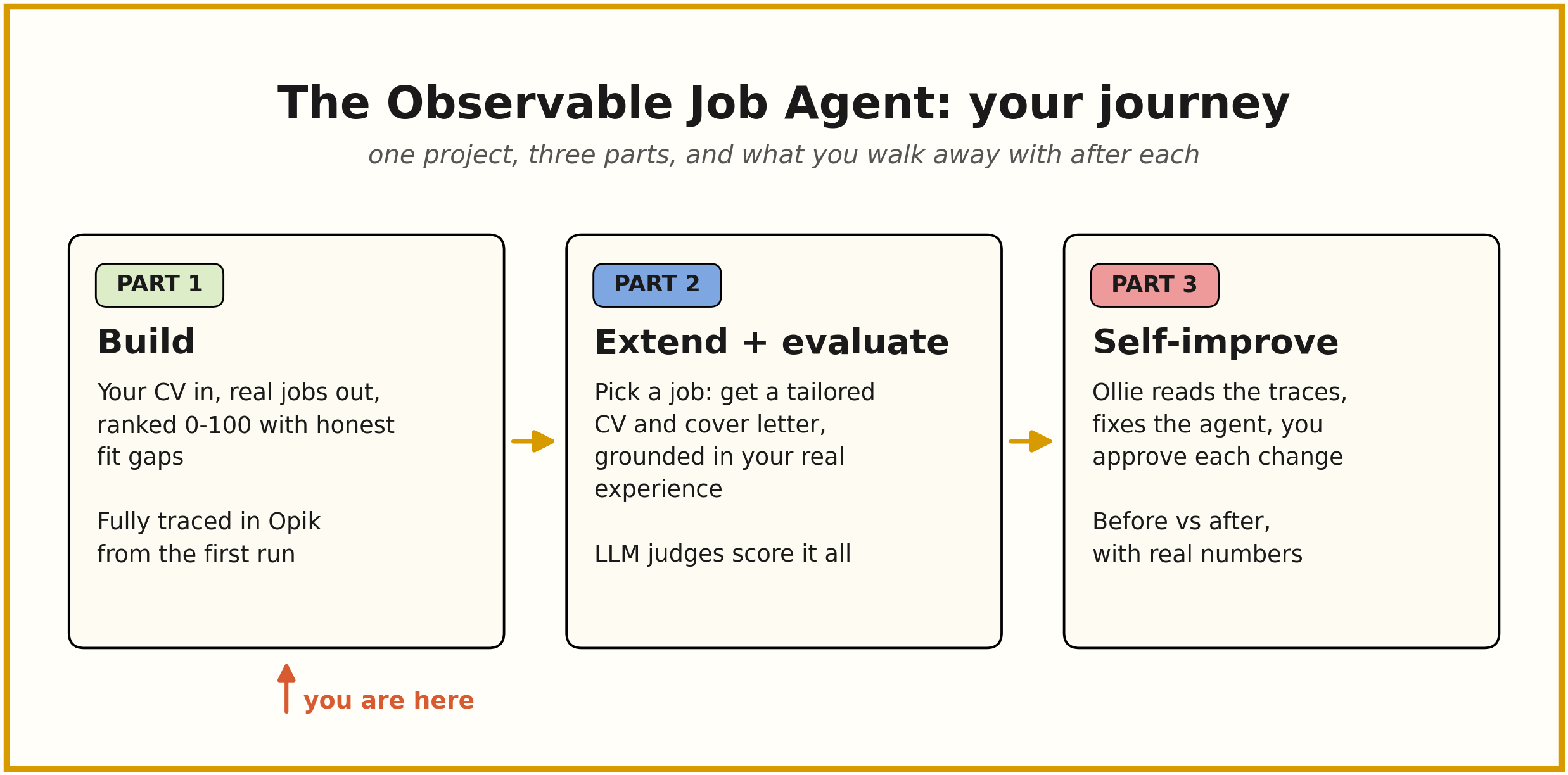
1. Part 1 (this post): Build. A working job-matching agent, traced in Opik from its very first run, plus a baseline batch that tells us honestly how good (and bad) it is.

2. Part 2: Extend, then evaluate. First we grow the agent: pick a job and it drafts a personalized cover letter plus tailored CV suggestions for that posting. Then we go deeper into the LLMOps: traces become datasets, we add LLM judges (including one that reads the attached CV PDF to catch fabricated experience), and we separate the checks you can verify from the judgments you can’t.

3. Part 3: Self-improve. Opik’s test suites, prompt optimization, and Ollie fix what Part 2 measured. We compare before and after with real numbers.

Want to set up while you read? Two links are enough to start:

• Code: https://github.com/jamwithai/observable-job-agent

• Opik (free account, for LLMOps): https://www.comet.com/signup

• JSearch API (free tier): https://www.openwebninja.com/api/jsearch

Clone the first, sign up for the second (its free). Full setup steps come later in the post.

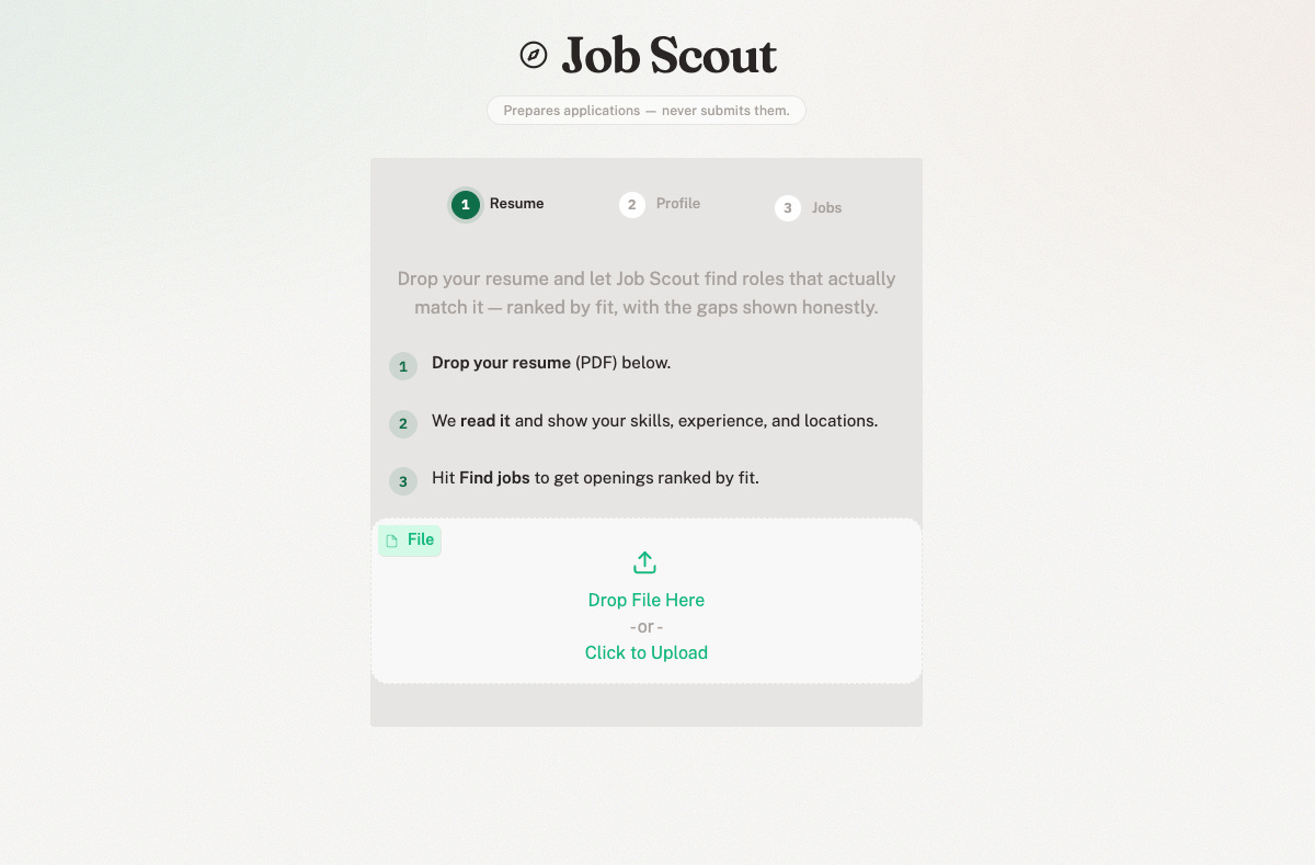
• Build Job Scout, a LangGraph agent: CV (PDF) in, ranked real job openings out

• Show real LLM-driven tool usage: the model chooses the search arguments, not our code

• Integrate Opik observability with one API key, one library, one line of code

• Version our prompts from day one so Part 3 can prove improvements later

• Run a baseline batch and document (not fix) every weakness the traces expose

• End-to-end agent: profile extraction, multi-source job search, batched fit ranking, a bounded reformulation loop

• Full Opik tracing on every run: span tree per node, auto-drawn agent graph, per-run cost, CV attached to the trace

• Gradio interface with streamed progress and a run footer (cost, latency, deep link to the trace)

• Multi-source job search (JSearch, Adzuna, Remotive, offline cache) that runs with zero API keys

Big picture: We are building the observable foundation. The agent works end to end, every run is measurable, and we finish with a written-down baseline of exactly how good (and bad) it is.

Complete job-matching agent with LLM tool usage, a conditional reformulation loop, and full Opik tracing from run one.

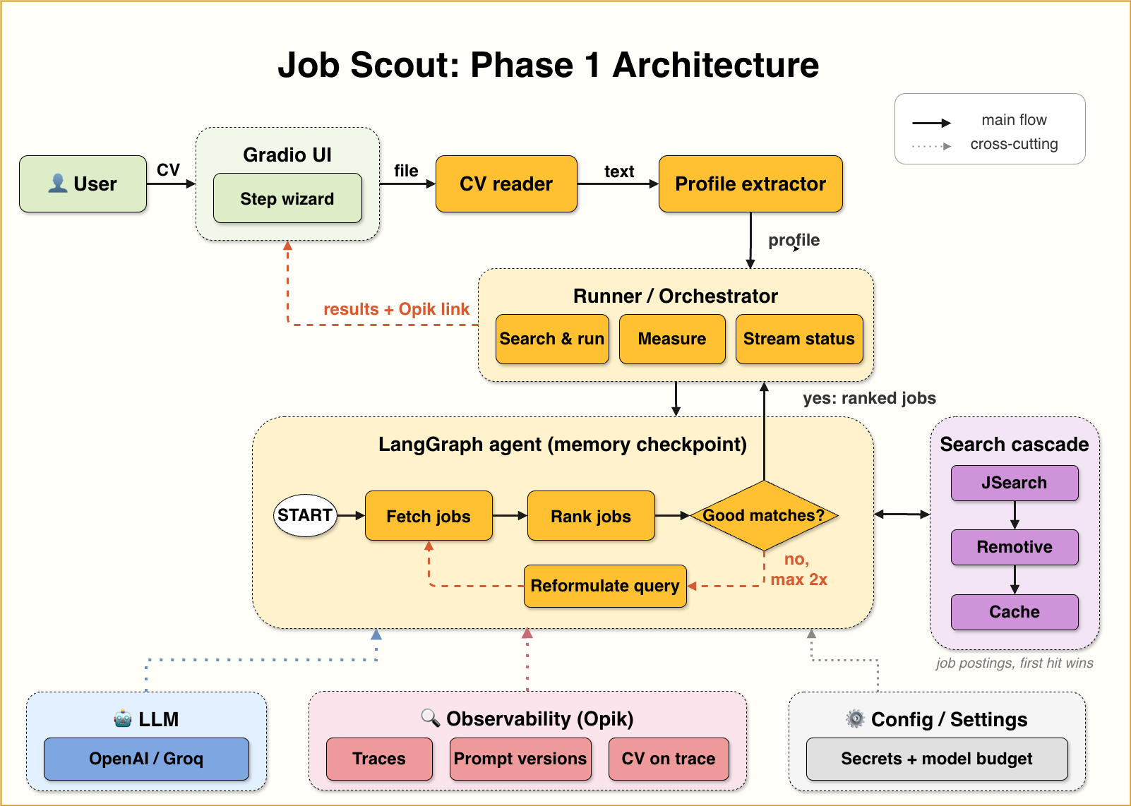
In one breath: your CV becomes a typed Profile. A LangGraph agent lets the model choose how to search four job sources, down to a keyless offline cache. It scores the results in batches, and loops once or twice to broaden the search if the matches are thin. Opik traces all of it.

We walk every one of those decisions in the next section.

One hard product rule: the human applies, the agent never submits. Auto-submitting breaks most job boards’ terms, and recruiters spot mass-generated applications quickly.

The real bottleneck is not clicking submit. It is the 30 minutes of tailoring per application. That is the part worth automating.

Could ChatGPT do this once? Sure. But you are not building a chat session. You are building a system that runs unattended, at a cost you control, with quality you can measure. Measure is the word this series is about.

The three prompts in this system are deliberately first-draft quality. No few-shot examples, no chain-of-thought scaffolding. Part 3 optimizes them against real metrics, and we want that improvement to be measurable, not already spent.

The map above is the what. This section is the how.

A LangGraph agent is three things, and no more:

• State: one typed object that every step reads from and writes to. The shared memory.

• Nodes: plain Python functions. Each takes the state, does one job, returns an update.

• Edges: who runs next. Most are fixed. One is decided at runtime by the model’s own output.

That last edge is the part that matters most.

State, nodes, and one edge the model’s output decides. Everything else is plumbing.

Now let us walk the lifecycle, one component at a time, in the order a run actually flows. The snippets are lightly simplified for reading; the repo is the source of truth.

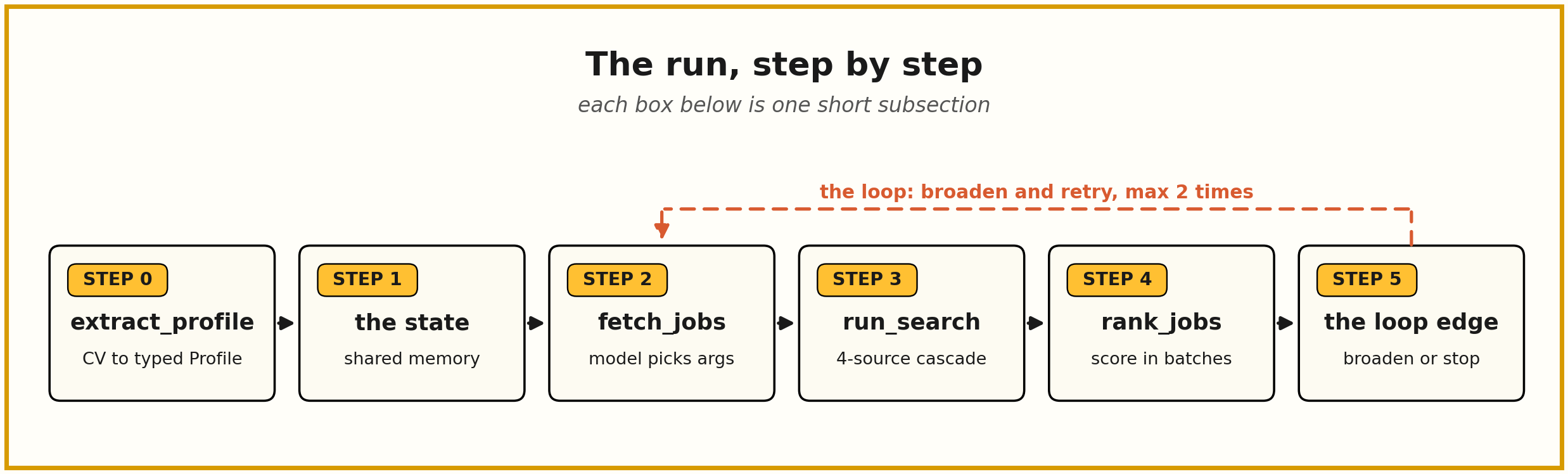
The first LLM call never touches the graph. extract_profile takes the raw PDF text and returns a Profile: seniority, roles, skills, locations, languages, a short summary. One structured-output call (the model must answer in the schema’s exact shape, not free text), and the schema does the validating.

Why a typed object instead of just text? Because every later step depends on this one. Free-form text would force each node to re-parse and guess (”was the location in there? spelled how?”).

A typed Profile gives every node the same guaranteed fields. If the model returns something malformed, it fails loudly right here, at the boundary, instead of quietly corrupting the ranking three steps later.

There is a bonus that pays off later: a typed output is a checkable output.
In Part 2 we evaluate extraction by comparing these exact fields against hand-written expected values. You cannot do that with a blob of text.

Why keep it out of the graph: the graph should do one thing, finding jobs. Extraction runs once and gets reused. The UI extracts, shows you the profile, then hands the same object to the search.

That means a cleaner graph and one fewer LLM call per loop.

This is the shared memory. Every node receives it, and returns a partial update that LangGraph merges back in.

total=False is doing quiet work. It lets each node return only the keys it changed, and lets the first invoke pass only the fields it has.

Three of these fields are about running the agent safely, not about the product. reformulation_count bounds the loop. llm_calls bounds the spend. jobs_sources becomes trace metadata, so a run can explain itself six weeks later.

This is the node that makes the “agent” word honest. We do not write the search query. We bind a search_jobs tool to the model, describe the candidate, and let the model choose the arguments.

Why it matters: the model reads a profile and decides “senior machine learning engineer, country DE, remote true.” Our code executes that decision and nothing more.

And because every run is traced, you can open any trace and watch which arguments the model picked. That is the difference between an agent you hope works and one you can inspect.

One search tool, and the model picks how to use it. Your code still drives the car, but the model reads the map.

There is a deterministic fallback if the model returns no tool call. We build a query from the profile’s roles and skills instead. An agent that hard-fails whenever the model skips the tool call is not a system you can leave running.

The tool itself is a cascade. Each source is tried only if the ones before it returned too few results.

Every adapter follows one rule: never raise. On a network error or a bad response it returns an empty list, and the cascade falls through to the next source. The last source is a committed offline cache of roughly 247 postings.

The payoff: make app works the moment you clone, with no keys at all. Remotive and the cache are fine for trying things out. Add keys when you want live, city-level results.

The postings come back, capped at 25. rank_jobs scores them in batches of 5, one structured-output call per batch. Each job returns with a fit score from 0 to 100, a short explanation, the skills that matched, and the gaps.

Why batched, rather than one call for all 25 or one call per job? Cost and reliability. Smaller structured outputs are more reliable, and 5 batches is a handful of calls, not 25.

It also leaves an obvious performance bug in plain sight. We come back to that when we read the traces.

After ranking, one function looks at the results and decides what happens next. This is the conditional edge, and it is the line between a workflow and an agent.

If fewer than 5 jobs clear a fit score of 60, and we have not already looped twice, the agent rewrites its own query to be broader and searches again. Otherwise it stops.

Two numbers define the behavior: the quality bar (5 jobs at 60+) and the hard cap (2 loops).

The conditional edge is what makes this an agent. The cap on it is what makes it a system you can leave running unattended.

Reaching the cap with thin results is not a failure. Some candidates genuinely do not match many open roles this week. Looping forever would just burn tokens.

The last piece ties everything together. Both the Gradio app and the baseline batch go through the same runner.py. It builds the tracer, wraps the graph, streams per-node status, and measures cost and latency in one place.

Why this matters: if the UI and the batch had separate run logic, they would drift apart. Your baseline numbers would then measure something users never experience.

One shared runner means the numbers we quote later come from the exact code path behind the screenshots.

That is the whole architecture: a typed profile in, a bounded loop where the model picks its own search, four job sources behind one tool, one shared runner. Small on purpose. The next section makes every piece of it observable.

Here is the entire observability integration. We are not compressing for effect. This is all of it.

Beat 1: a key and a library. Sign up for free on Opik (the free tier covers everything in this series), install the library, and add your keys:

Beat 2: configure once.

Beat 3: one line to trace the whole graph.

Notice thread_id in that snippet. It ties multiple invocations together as one conversation, which starts to matter in Part 2 when tailoring reuses the same thread.

No decorators sprinkled through the codebase, no manual span bookkeeping, no changes to any node.

Every node becomes a span, every LLM and tool call nests under its node, and the whole thing lands in a dashboard.

One key, one library, one line. The barrier to real LLM observability in 2026 is lower than the barrier to setting up structured logging.

We are aware that “one line” claims usually hide a footnote. Here the footnote is honest: the one line gets you tracing. Making the telemetry production-grade (identity, attachments, graceful degradation) took a thin wrapper module.

A fair question from LangGraph users: why not LangSmith? It works well if you stay inside the LangChain ecosystem. We picked Opik because it is framework-agnostic and open source, so when your stack changes, your observability does not have to. For a project we are telling you to extend, that matters.

And frankly, we really loved in Opik

Run the app once, open the project in Opik, and this is waiting for you.

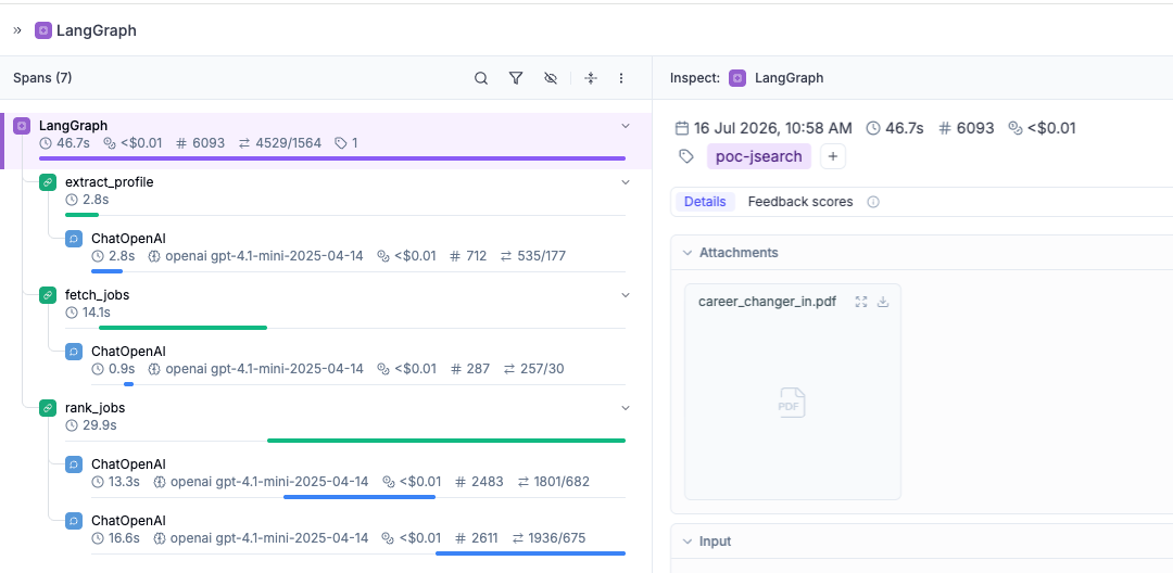
A span tree per run. Each graph node is a span; the LLM and tool calls nest beneath it. You can watch fetch_jobs issue its tool call, see which arguments the model chose, and see exactly what the ranking call received.

The agent graph, auto-drawn. Opik extracts the graph structure and renders it in the trace sidebar. The fetch → rank → reformulate loop appears without us drawing anything.

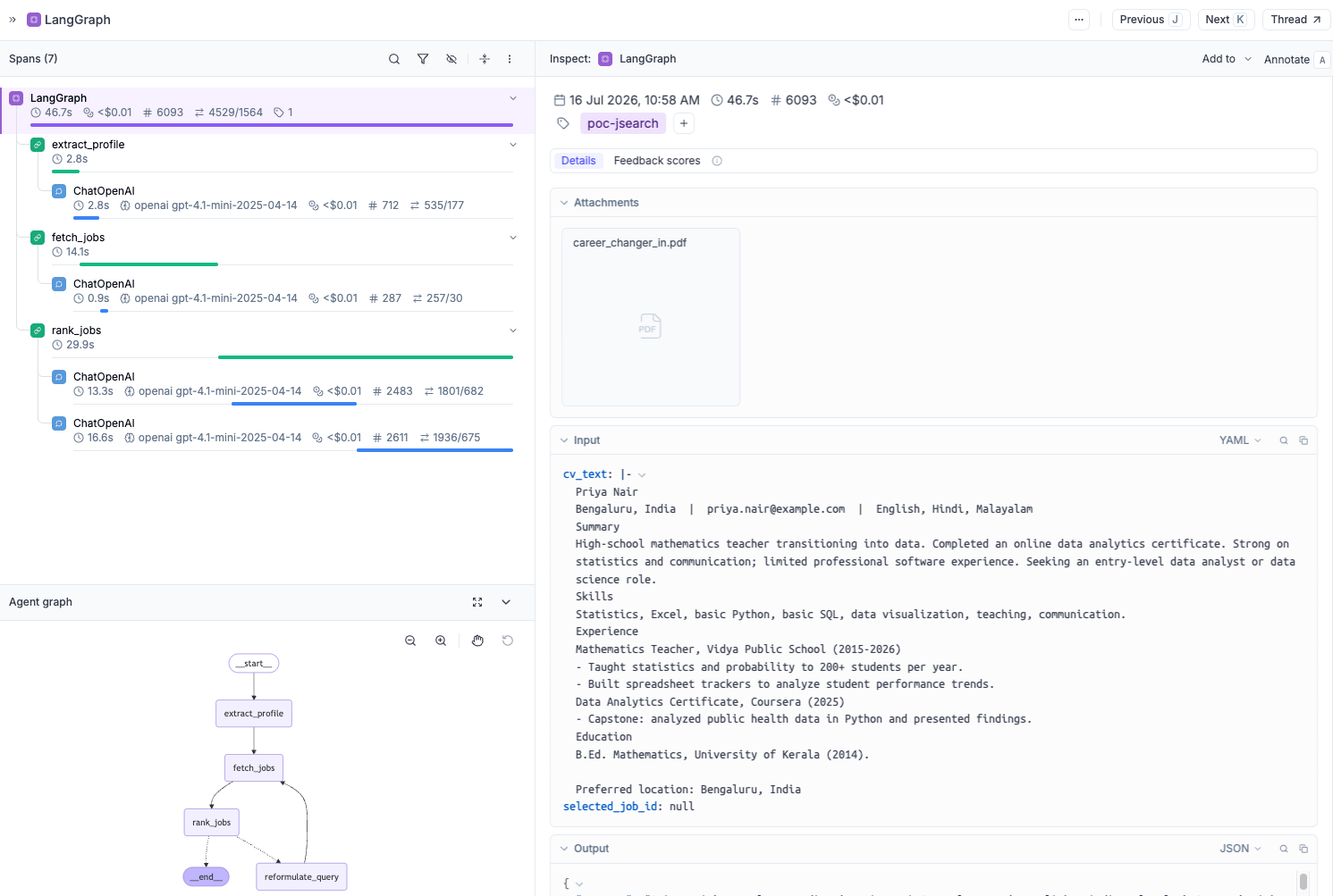
Per-run cost, computed for you. For priced models (OpenAI, Anthropic, Google), Opik computes exact per-run cost from token counts. Our UI footer shows a local estimate; the trace holds the real figure.

Two things to know so you don’t file a bug report: free models (Groq, Ollama) correctly show $0.00, and the footer is an estimate by design.

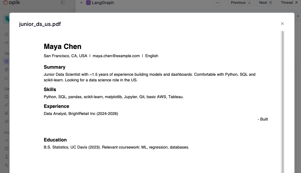
The CV, attached to the trace. We upload the source PDF onto each run’s trace. Today that is nice for debugging.

In Part 2 it becomes important: Opik’s LLM judges can reason over trace attachments. That is how we will check generated content against the actual CV to catch fabricated experience.

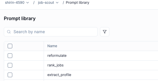
Prompts as versioned artifacts. Our three prompts live as plain Python constants in the repo, the source of truth. A small register_prompts() helper mirrors them into Opik’s prompt library and creates a new version whenever content changes.

This feels like extra ceremony today. In Part 3 it matters: the optimizer needs that prompt history to show whether a change actually helped.

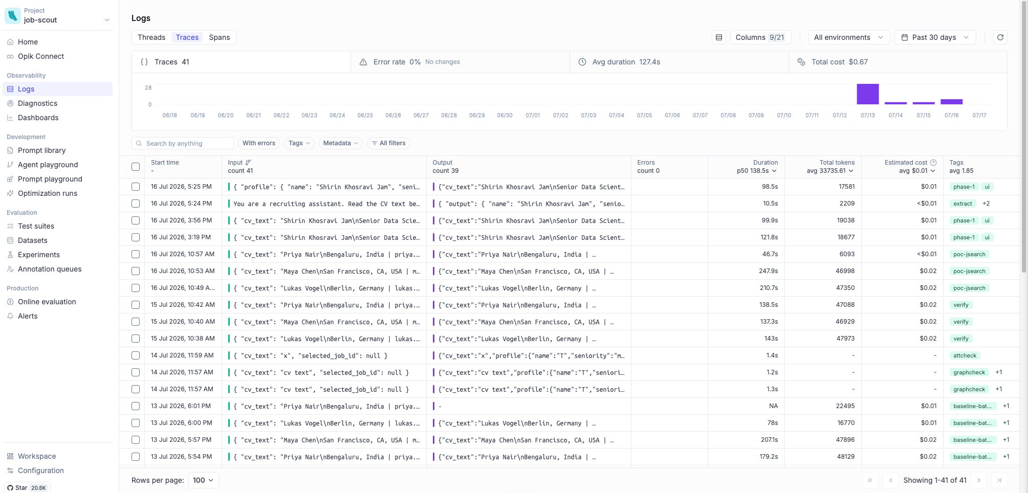
Here is where tracing from day one starts paying off. Before writing Part 2, we ran a baseline batch: the repo’s synthetic example CVs (fixtures) crossed with target locations, plus deliberately hard cases (a career changer, a non-English CV, a profile matching almost nothing).

19 runs on gpt-4.1-mini, all traced and tagged baseline-batch.

The numbers:

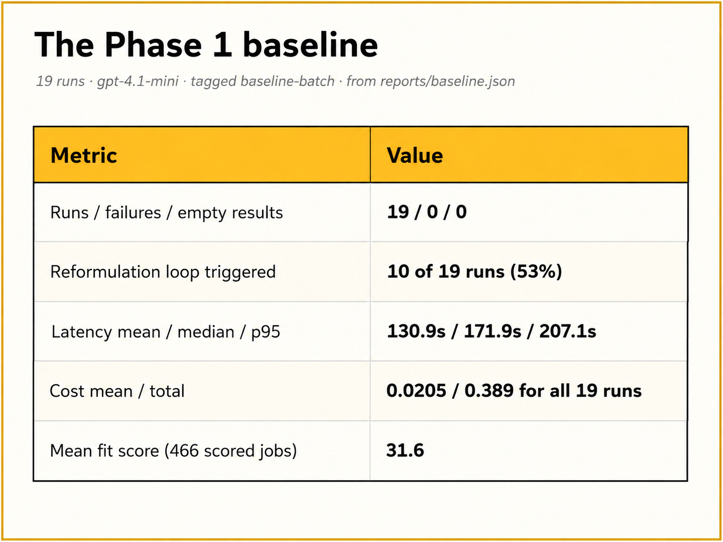
(A typical single UI run on the default gpt-4o-mini, without a reformulation loop, takes around 90 seconds. The batch medians are higher because they use a different model and include the loops.)

And the traces surfaced five concrete weaknesses. We documented them and, deliberately, fixed none of them:

1. Location constraints get ignored. One CV run with US, UK, Germany, and India hints produced the same Remotive-only result set each time.

2. The reformulation loop fires constantly and rarely helps. Weak profiles loop to the cap and barely improve their results.

3. Reformulation dominates cost and latency. Looping runs cost around $0.030 and take 170–210s, versus $0.007–0.011 and 55–98s without. Roughly 3× on both axes, for marginal gain.

4. Ranking skews low and compresses at the top. Mean of 31.6, strong profiles plateauing at a flat 90. A first-draft rubric that barely separates good matches from bad.

5. Nothing verifies matched_skills grounding. The ranker claims skills matched; no check confirms they appear in both the profile and the job text. A fabrication risk, and it becomes a named metric in Part 2.

And in fairness to the agent: zero crashes and zero empty results across 19 runs. The error handling and the offline cache held up.

Measure, don’t fix yet. Every one of these five weaknesses is now a baseline number. When Part 3 fixes them, we get to prove it instead of claiming it.

The spans also exposed a performance bug: rank_jobs scores its batches in a serial loop, one blocking LLM call after another, even though the batches are fully independent. The span waterfall makes the fix obvious. Concurrent batch calls would cut ranking time from the sum to roughly the max.

We are leaving it slow on purpose, because this one is Ollie's job. In Part 3 we point Opik's trace-reading assistant at exactly this waterfall and let it diagnose and implement the fix, with the before/after spans as proof.

📓 Code location: https://github.com/jamwithai/observable-job-agent

📓 Interactive Tutorial: notebooks/phase1_walkthrough.ipynb

• Complete setup verification with health checks

• Step-by-step run of the agent with a fixture CV

• Reading your first trace in Opik

• Reproducing the baseline batch (with a --limit flag to keep it cheap)

📁 Key Files:

src/job_scout/tracing.py - all Opik wiring in one module

src/job_scout/runner.py - run orchestration shared by UI and batch

src/job_scout/graph/graph.py - the StateGraph, thresholds, and the loop

src/job_scout/tools/jobs_api.py - the four-source search cascade

scripts/run_batch.py - the baseline batch harness

📚 Documentation:

docs/opik_setup.md - setup plus “what gets traced”

docs/extending_sources.md - how to add a job source (and why there is no LinkedIn scraper)

Prerequisites:

1. Clone the repo and sync: uv sync --all-groups

2. Copy config: cp .env.example .env

3. Keys: OpenAI (live ranking), Opik (tracing), JSearch (live jobs).

Every key below has a free path. Grab the ones you want, paste them into .env, done. And remember: these are simply the sources we ship with. The JobSource design expects you to add more later, so treat this list as the starter pack, not the menu.

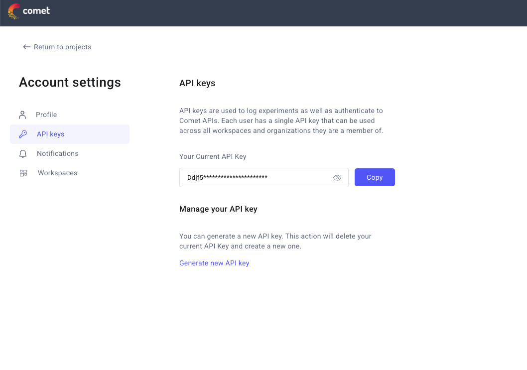
1. Opik (tracing, free tier): sign up at comet.com, then your API key lives under your profile → API Keys. Workspace name is shown on the same page.

2. OpenAI (ranking model, ~$0.50 for this whole post): platform.openai.com → API keys → Create new secret key. Alternative you can use Groq or any other provider’s free tier.

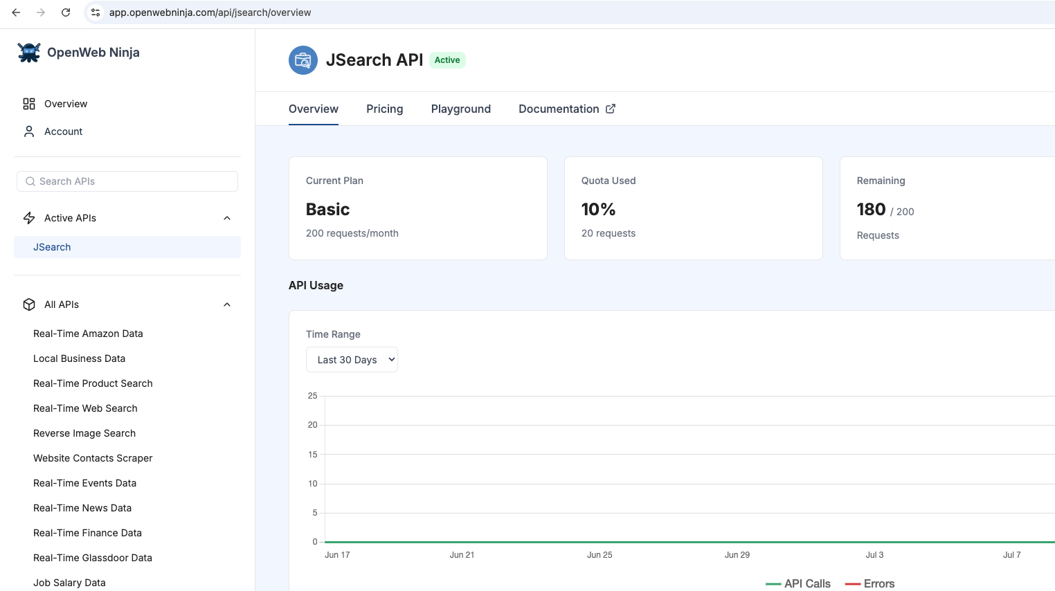
3. JSearch (live job listings, free tier): it is distributed through RapidAPI. Search “JSearch” on rapidapi.com, subscribe to the free Basic plan, and copy the key from the endpoint playground.

Three ways to test:

1. The test suite

make test   # 32 tests, no network, no credits spent

2. The Gradio interface

make app
# upload a fixture CV from data/fixture_cvs/

3. The baseline batch

make batch  # add --limit 3 for a cheap dry run; full batch costs ~$0.40

Total cost to reproduce everything in this post: under $0.50.

Let’s be explicit about what this is: a base, not a product. We build the foundation step by step in this series; extending it and adapting it to your situation is the part that belongs to you. The codebase is deliberately structured for exactly that, and here is where we would start:

• Add job sources beyond the ones we ship. JSearch, Adzuna, and Remotive are our starter pack, not the menu. The JobSource protocol is one class with one method (docs/extending_sources.md walks through it), so a local job board with an official API, a niche board for your field, or a company careers API drops in cleanly, and the cascade handles the rest.

• Tune the fit rubric to your field. The ranking prompt is a plain constant in graph/prompts/rank_jobs.py. Care more about remote-first? Weight it. Switching fields? Tell the ranker how to treat transferable skills. (And since prompts are versioned in Opik, you can check whether your edit actually helped. Part 3 is all about that.)

• Swap the model. SCOUT_MODEL is one env var: OpenAI, Groq for free, Ollama for fully local. No code change.

Whatever you build on top, the tracing comes along for free. That is the point.

Next part, on both fronts:

Extend the agent: pick a job from your ranked list and the agent prepares your application: a personalized cover letter plus tailored CV suggestions for that exact posting, grounded strictly in what your CV actually says. Technically it is one new tailor node behind a conditional entry router, reusing the same checkpointed thread; the schemas already exist in the repo, so the trace format stays stable. (And yes, the agent still never submits anything. It prepares; you apply.)

Deepen the observability: the baseline traces become evaluation datasets. We add online evaluation rules and LLM judges, including the PDF-attachment judge that reads the CV on the trace, and we draw the line between metrics you can verify deterministically and judgments you have to treat with skepticism.

Follow Along: This is Part 1 of 3 of The Observable Job Agent series.

Let’s go 💪

If you enjoyed this read, do share it with your colleagues and team :)

Until next time. 💚