Rails and Roads By the Slide Rule

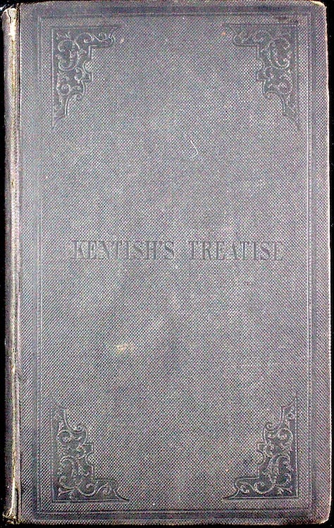
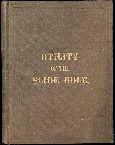
I’ve seen copies or images of many old books on the use of slide rules in the trades. A few examples of the interesting books from the 1800s that I’ve been able to acquire and examine first hand have been, A Treatise on a Box of Instruments and the Slide-Rule, by Thomas Kentish (1847), Treatise on Instrumental Arithmetic, or Utility of the Slide Rule, by Arnold Jillson (1874), and a booklet entitled, The Mechanics’ Slide Rule, and How to Use It, by Fred T. Hodgson (1881). The first book talks primarily about the Engineer’s rule (or, Soho rule), or, as Kentish refers to it, “… that in which the line D commences with unity.” About midway through the text, after discussing other instruments, he spends 10 pages or so discussing this slide rule and how to set up basic calculations, and then provides several dozen pages of examples and sample problems, all using a Soho-style slide rule.

Jillson’s book, on the other hand, is divided into two major parts — the first talks about the slide rule “where the figure 1, on the D line, is found in the middle” (i.e., the Carpenter’s rule), while the second part describes the slide rule where “the figure 1, upon this instrument, on the D line, is found at the end at left hand” (i.e., the Engineer’s rule). In each of these cases, the A, B, and C scales are all 2-decade logarithmic scales, with B and C being on the slide, while the D scale is a 1-decade log scale.

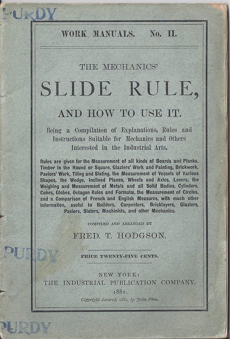
In Hodgson’s 1881 text, part of a series of Work Manuals for mechanics, he describes the use of “the Mechanic’s slide rule”, which, it turns out, is actually referring to what we now call the Carpenter’s rule. In the 1880s, a “mechanic” was a person that used tools to make or repair things, and here he was introducing to the reader how to use a by-then fairly common Carpenter’s rule for use in many other trades besides logging and carpentry. The several few pages of the text cover the general topic of how to read the scales and set ratios on the device. It then goes into a large number of specific numerical examples using this style slide rule, most of which only use scales A and B. Only in some examples of timber calculations does he use scales C and D.

The last three pages of the 29-page text, however, contain the section titled, “The Engineer’s Slide Rule”. Here Hodgson talks about how much more convenient this rule can be for the problems already worked. But, for further information, he refers the reader to other sources, particularly Kentish and Jillson!

By the early 1900s, as slide rules with the Mannheim scale arrangement began to supersede those found on the Carpenter’s and Engineer’s rules, the texts and manuals I’ve come across appear to have changed their approach. The earlier books primarily consisted of lists of problems related to their specific trade, such as how to compute the number of board-feet in a log, or the weight of a metal piston, etc. The user would simply look up the problem they wanted to solve and follow the example step-by-step, inserting the relevant numbers for their own case. In essence, it was simply a set of recipes for the user to look up when a particular calculation needed to be performed.

But the later texts by Charles Pickworth, William Cox, and many others starting from, say, around 1895-1910, seem to have placed more emphasis on the general computational methods using a Mannheim slide rule, such as how to perform basic multiplication and division, how to find roots, squares and cubes, raise numbers to arbitrary powers, use scales of trig functions, and so on. The chapters of the new texts were not tied to any particular trade, though many uses were examined, and the sample calculations emphasized the array of typical numerical expressions that needed evaluation. This trend illustrates to me the transformational influence of the invention of Mannheim’s scale set, with it being viewed as a general computing device, and not simply a tool with scales pertinent to one particular industry.

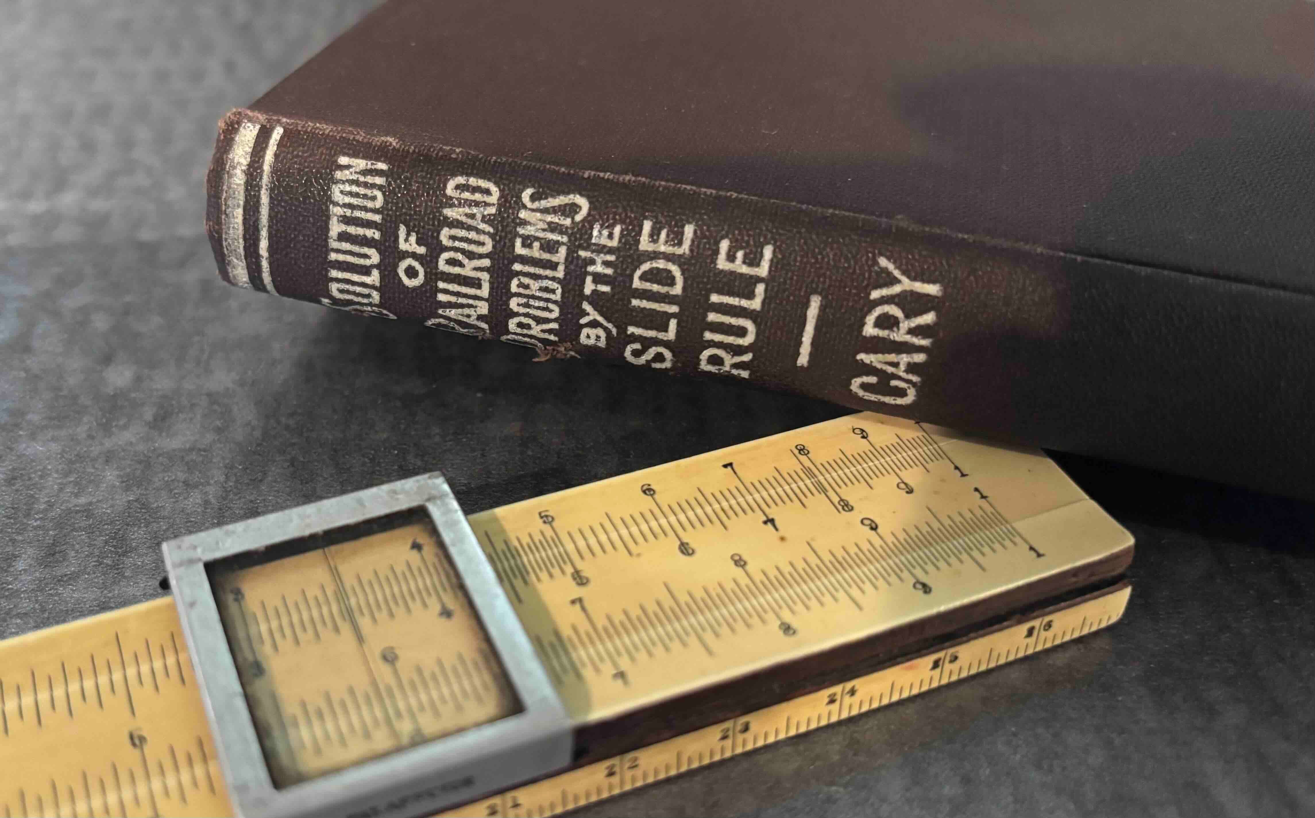
With apologies for the windy discussion above, all of this came to my mind when I was drawn to a book that I found recently with the title, Solution of Railroad Problems by the Slide Rule, by E.R. Cary (1913). The book, also available online, more or less assumes the reader understands how to use the Mannheim slide rule, perhaps learned from the texts by Pickworth, Cox, and so on. But this interesting little book of 136 pages delves into the basic calculations, mostly involving geometric ratios and trigonometry, of the curves and other features found in railroad design. The book introduces an engineering design subject through basic mathematics, and many of the various problems examined come with explicit instructions for performing them using a Mannheim slide rule.

The following gallery shows images of the table of contents:

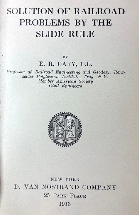
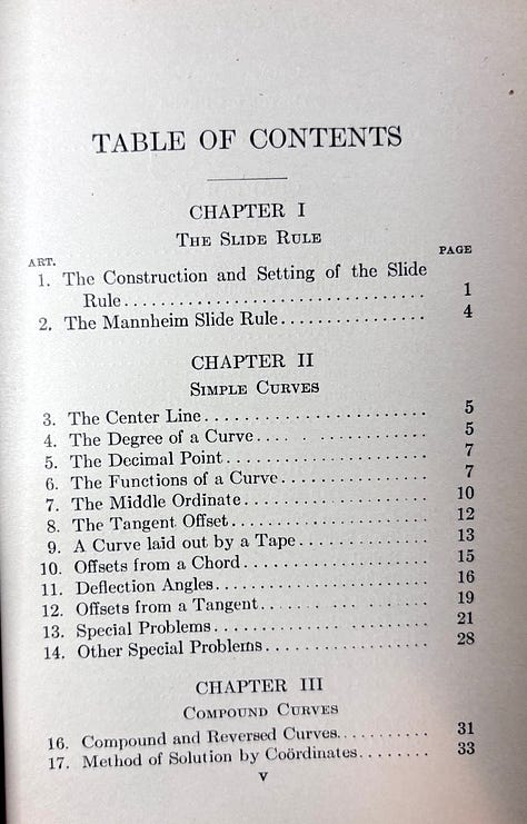
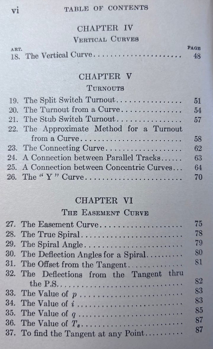
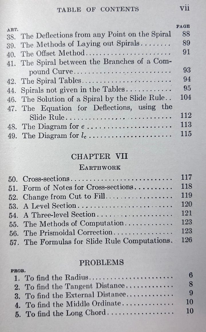
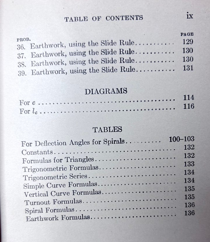
After a short 4-page review of the basic Mannheim slide rule, Cary goes directly into the equations used to lay out arcs, how to join arcs of varying radii, how to design a switch to move a train from one set of rails to another, and so on. It spends very little time teaching the terms used in the railroad industry, so I suspect it was meant to be a reference or textbook for those already in, or going into, the trade. Below I want to go through a few examples to get a flavor of the style of the book, and to illustrate a few items I found interesting.

Embedded in the text are about 40 worked problems. Here is an excerpt from two early problems in the text (Problems 2 and 3) which explains how to use the Mannheim rule to perform the calculations:

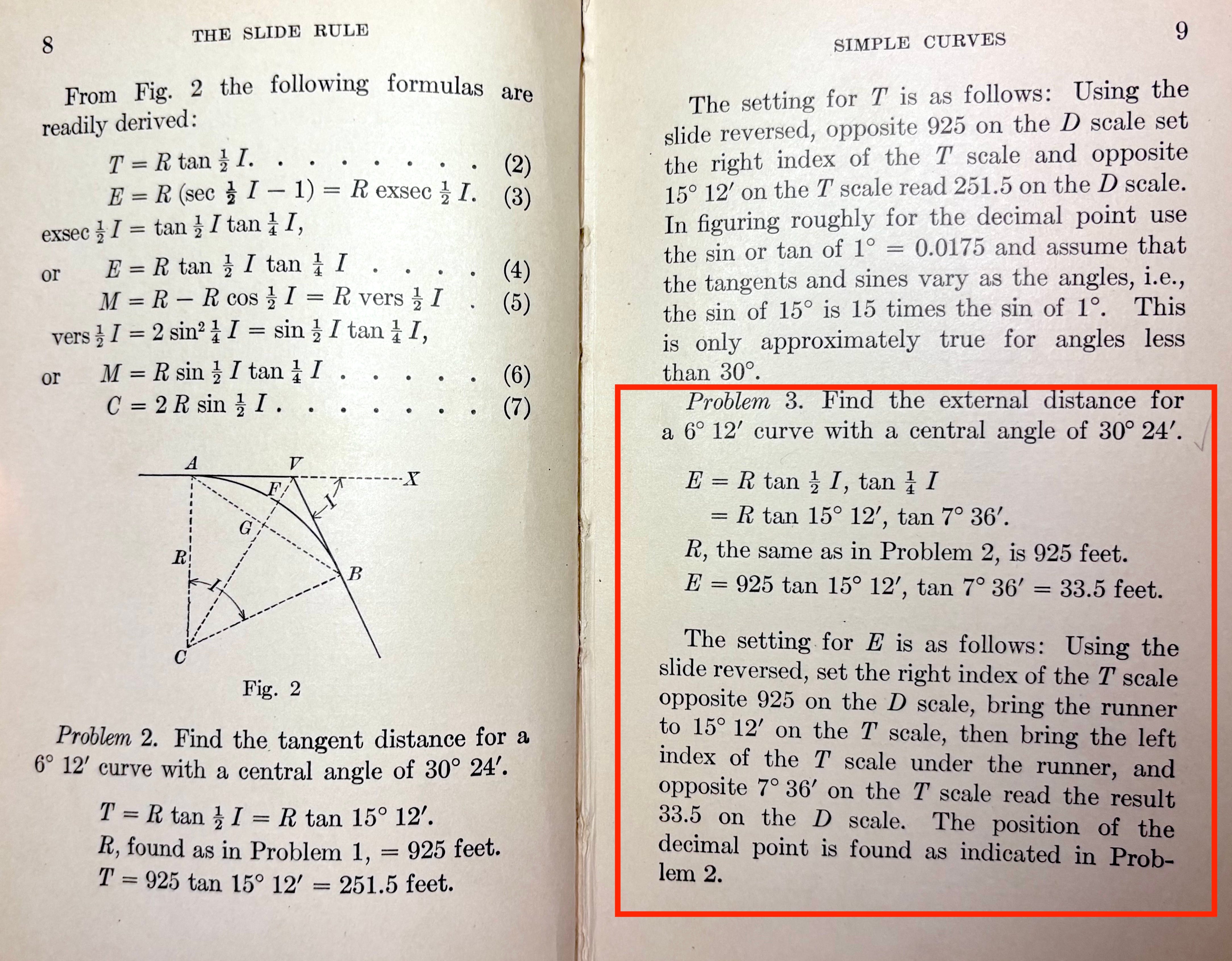
The calculation of the distance, referred to as “E”, between points V and F is computed in Problem 3 on page 9 (see rectangle). Note the use of the comma to signify multiplication of the two trig functions, a notation I hadn’t seen used before. Also note the use of D as the primary scale for the calculation, rather than A as in other problems found in the earlier texts. We’ve discussed in earlier posts how in the early 1900s the A/B scales were often thought of as the primary scales for calculations, with the C/D scales eventually taking over this title. And in fact, within the Preface of this book, the author states, “Where it is possible, the solution of the problems should be made by the use of the C and D scales of the Mannheim slide rule on account of their greater precision.”

On the other hand, using the D scale in this particular case may have been obvious to those trained in using the Mannheim, as the T scale was traditionally tied to C/D, while the S scale was tied to A/B. This was due to the fact that the T and D scales are found next to each other when the slide is turned over. So, starting with D to multiply a number by the tangent of an angle (or two) was probably natural to a user of that time for such a circumstance.

If you re-read the original text of problems shown above, they start out by saying “Find the tangent distance…”, or “Find the external distance…”, of “a 6^o 12’ curve with a central angle of 30^o 24’. ” This last phrase took me a while to figure out what they were describing. Why are there two angles, and to what are they referring?

What I learned was that in the actual surveying of such curves, the standard section of railroad track is one in which the chord between two survey stations is taken to be of length 100 feet. Thus, when the book talks about the “degree of the curve”, which they call D, it is the expected angle created through a curve that has a half-chord length of 50 feet. Using Fig. 2 in the book, shown in our earlier image, this amounts to

Since such angles are generally small over the length of 100 feet, then if D is expressed in degrees, we can convert to radians and have as a good approximation,

So, in 1913 at least, rather than talking about the radius of curvature of a segment of track, the “Degree” of the track, D, is often quoted. But this expression really is all about setting the radius of curvature, R. Throughout the book, a problem or equation requiring R is often times expressed in terms of D, with this relationship implied.

So, in the above phrase “…a 6^o 12′ curve with a central angle of 30^o 24′,” the first angle tells us that the radius of curvature is R = 5730/(6+12/60) = 924 feet, and the second angle is the actual number of degrees of the arc being made using that radius.

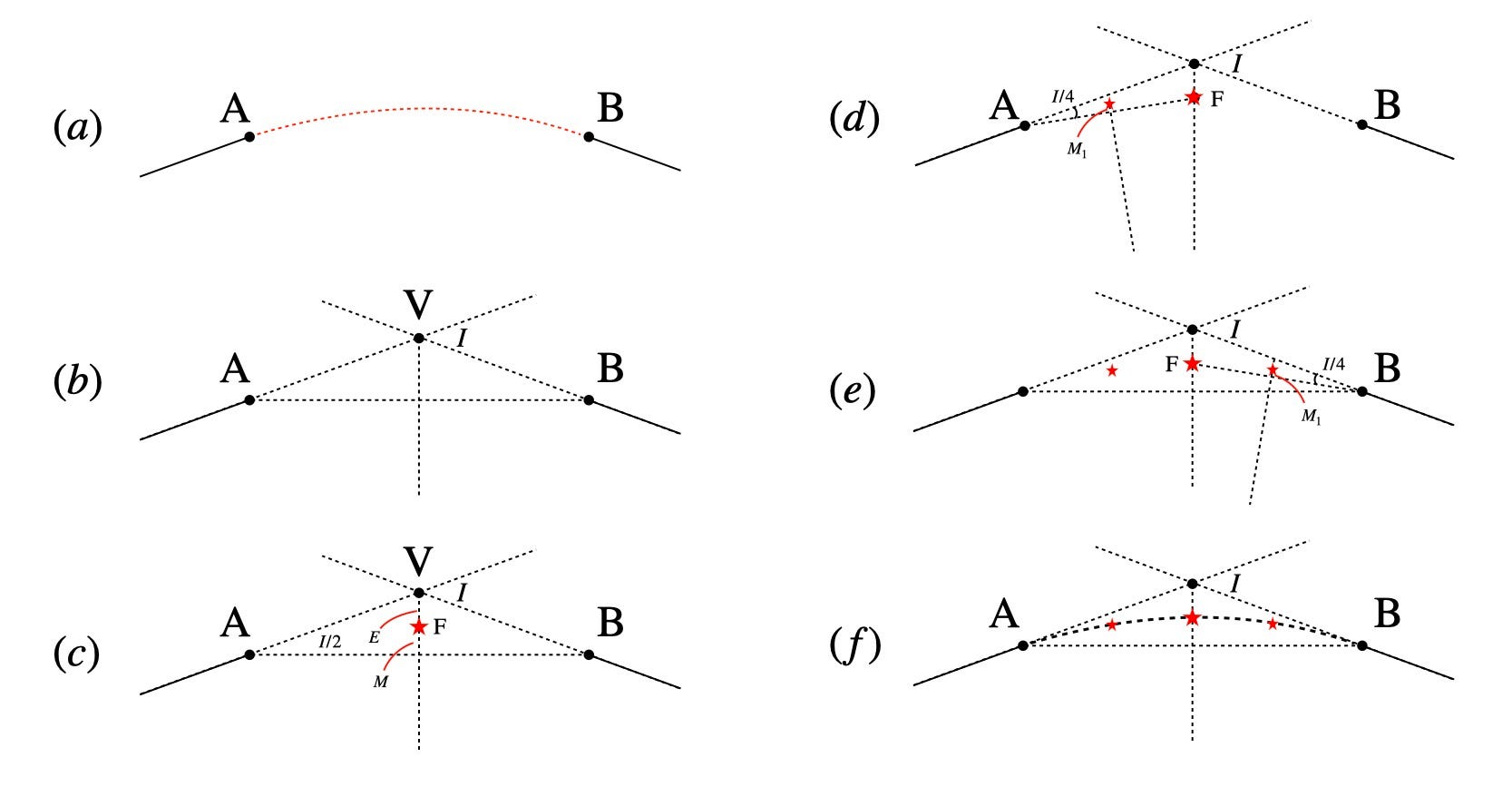
Again, from Fig. 2 in the text above, and the image below, one can see the general construction of the circular arc joining two straight lines (a), starting and ending at points A and B. In the real world, the procedure might go as follows. By extending the two lines, the intersection point V of the two tangents through points A and B is found (b), and the distance E from point V to the point F on the arc, or the distance M from the chord to point F, is then computed (c). Once the point F is found, the process can be repeated by drawing chords between points A and F and between points F and B and then finding two new points on these portions of the arc (d and e), and so on, until a good description of the arc is formed (f). This would involve a repeated calculation, in which the angle used is cut in half for the next iteration.

Problem 3 on page 9 in the image of the book above shows the process for computing the external distance E between points V and F, using a Mannheim slide rule, through standard computational procedures. The essential calculation can be performed in one of two equivalent ways. One either could use

which is easier to obtain geometrically,1 or, equivalently, through the use of trig identities, we can re-write the expression in the form,

This is the form that is executed in the example in the text. It is better suited for the slide rule, as it does not require a subtraction before multiplying by R, nor does it require subtracting I/4 from 90 in order to find the cosine of the appropriate angle using the sine scale.

Many of the calculations being described in the book have to do with “switching”, where trains are guided from one section of track onto a different section of track. The general topic is introduced in Chapter V. As one would expect, this deals with many variations of arcs and tangents and thus relies heavily on the type of calculation shown above. A few sample pages are shown below for illustration, but each sub-topic often continues for many pages.

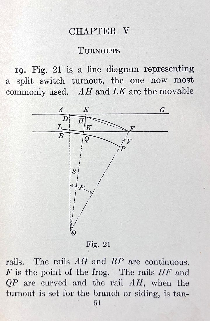
Cary goes through the development of the computation of angles and distances in several of these standard layout situations for rail systems. In most instances, examples of the step-by-step calculations using the slide rule are provided.

In Chapter VI, titled “The Easement Curve”, the development of a 3-dimensional “spiral” is discussed, where the outer rail is gradually raised with respect to the inner rail over a certain distance at the beginning of the curve. The final angle that results is chosen in order to counterbalance the centrifugal force experienced by passengers and cargo while traversing the curve.

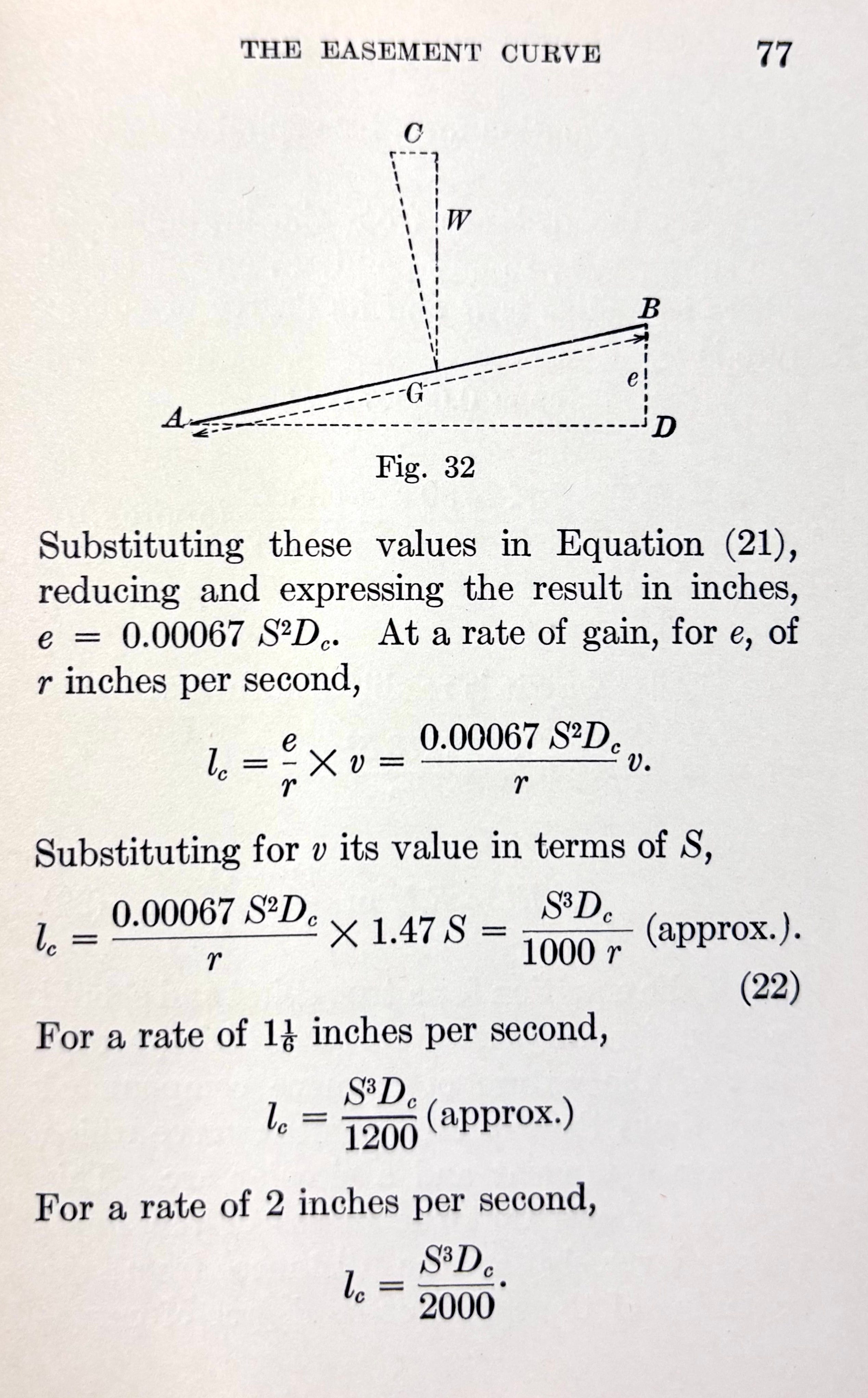
It is in this discussion that we find the introduction of squared and cubed variables in the equations, which brings about the use of the C/D scales in conjunction with the A/B scales on the slide rule.

The figure above illustrates a cross section of track where, here, the points labeled A and B represent the banked set of rails, with the outside rail elevated by a distance e. The constant distance between the rails A and B is called the gage, G. For a particular radius of curvature, and for a particular train speed, there is an ideal banking angle that compensates the centrifugal force, illustrated in the above figure. However, when entering into such a curve from a level surface, an abrupt change to this angle is certainly undesirable. It would be better, at least for the sake of the train’s contents, to ease into the desired condition.

In the text, it is noted that a gradual rate of increase in elevation of the outside track by 2 inches per second goes essentially unnoticed, or is certainly tolerable, by a passenger on the train, and this rate, r = 2 in/sec, was a typical value for this requirement of the system. So as the train enters the curve, the outside rail is gradually raised at this rate until the desired final value of e is reached, which is then held until coming out of the curve. At the other end of the curve, a reversed spiral brings the track back to level. To approximate the length of track over which the transition is made to the final banking angle, the rate, r can thus be expressed in terms of the overall length, l_c, of the spiral section over which the rail was raised or lowered by an amount e while entering or exiting the curved section. If the speed of the train is v, then

From the image of page 77 shown above, the ratio of the centripetal force, C = mv²/R , to the weight of the train, W = mg, is found to be equal to the ratio of e to the gage G of the track:

where m is the mass of the train and g is the acceleration due to gravity. And so, solving for e, we get the final desired elevation of the outside track relative to the inside track,

Thus, the spiral sections at the beginning or end of a curve, through which the outer rail is raised or lowered by a total amount e, should be approximately of length

The text goes on to show how to arrive at a more appropriate formula for a better spiral curve that actually eases into the easement, but we won’t go through that here. Meanwhile, Problem 33 on page 104 of the book provides a calculation of a spiral length using the above equation, with the steps used on the Mannheim provided on page 105.

First, though, the equation is simplified through the use of standard parameters such as, g = 32.2 ft/s², G = 4.71 ft (the standard gage), D = the “degree” of the circular curve in degrees, R = 5730/D = turning radius in feet, and S = the speed of the train in miles per hour going through the curve. That is, if we convert the units of our variables into a common set of feet and seconds, then the length l_c in feet, to within a few percent, turns out to be

which itself makes for a great slide rule problem to work out (hint, hint).

Back to the calculation described in the book, the determination of l_c is described at the bottom of page 104, using this last formula. The steps to do the calculation using the slide rule begin at the top of page 105.

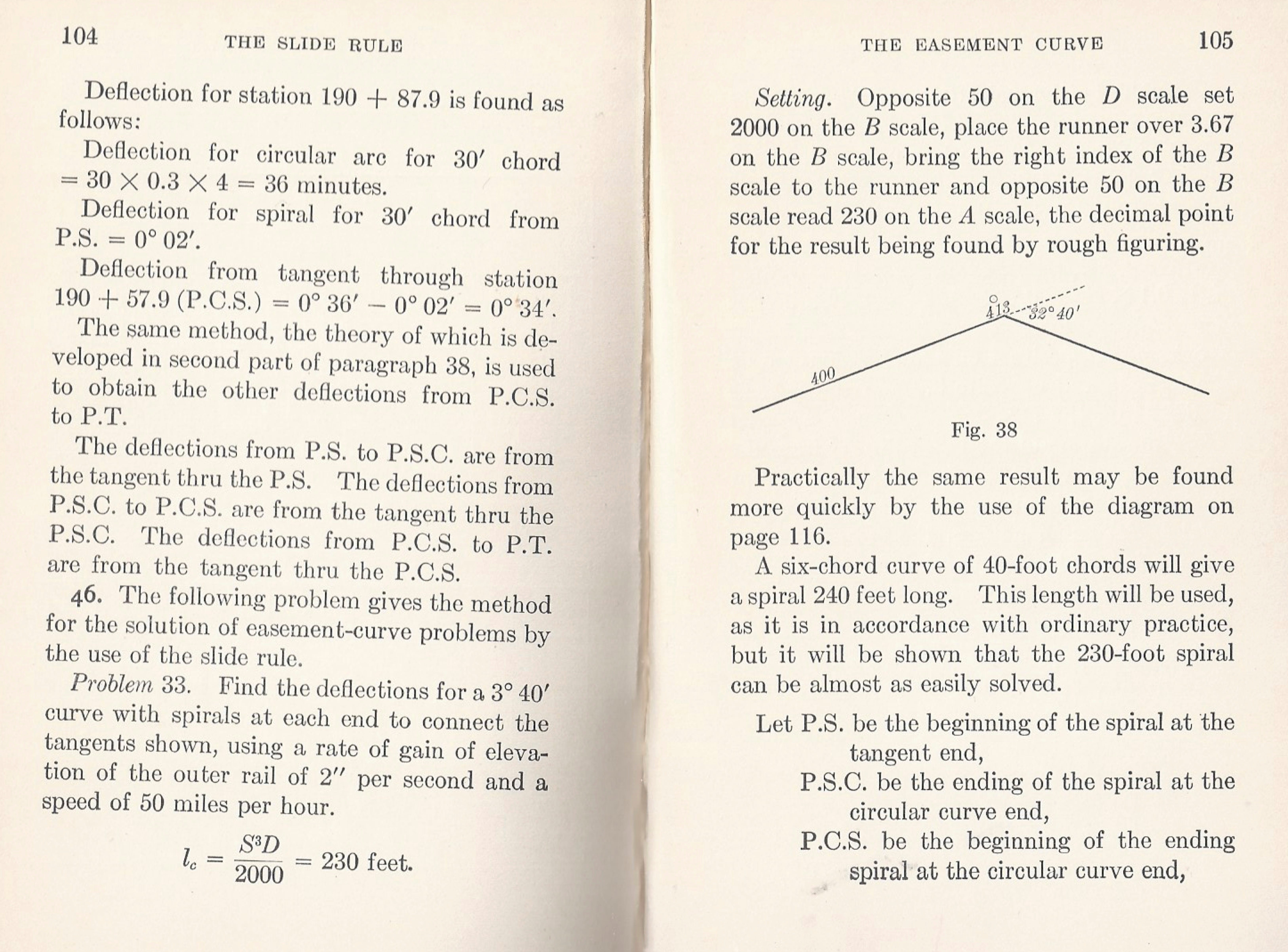
Let me expand slightly on the explanation, by embellishing the steps a bit (and please feel free to follow along on your slide rule):

• First, always, estimate the answer:

  • (50)³ × 4 / 2000 = 5³ × 10³ × 4 / (2 × 10³) = 125 x 2 = 250.

• Then, to perform the calculation on the slide rule:

  • We want to compute 5³ × 3.67 / 2

  • Setting the cursor to 5 on D, its square, 25, is above on A.

  • Aligning 2 on B to the cursor is dividing, thus 5²/2 is at the index on A.

  • Moving the cursor to 3.67 on B is multiplying; here 3.67 is the angle D = 3^o 40’ expressed in decimal degrees. This yields 5² × 3.67 / 2 at the cursor on A.

  • Next, move the index to the cursor hairline, thus preparing for the final multiplication.

  • This is performed by moving the cursor to 5 on B, thereby multiplying by our third factor of S, and provides the final answer under the cursor on A. I find the digits 230, which from our estimate says the answer is, indeed, 230.

  • Our dimensional analysis shows that the final answer will be in units of feet: l_c = S³D/2000 = 230 ft.

All in all, this is a very interesting book, small in size but with an enormous amount of detail into the computations that took place around the beginning of the 20th century relevant to the railroad construction business, all brought about by basic slide rule calculations. As interesting as I found the railroad design aspects, I found the examples of the calculations just as interesting and enlightening. Many examples include the preparations made through trig identities and various approximations that could often be made before executing the calculation. I remember asking my High School Trigonometry teacher, Ms. Hawk, “why did we have to derive all of these identities for homework?” She told me that re-writing an expression by using trig identities could often make the final numerical calculation easier to perform. She was right (of course), particularly when computations were made by using a slide rule or a book of logarithms.

Many of the same types of calculations described in our railroad design book are directly applicable to the design and construction of roads and highways. I found that while the calculations are basically the same, the approach can be a bit different in certain aspects. For instance, from the start of the development of the railroad, the standard in the surveying and layout of a curve would be to place stations 100 feet apart along chords of the curve. The next chord would be at an angle D degrees with respect to the previous chord. Then offsets from those chords would be generated, as described above, to create the actual curve.

In U.S. highway construction, 100 feet has also been a standard distance, but in this case along the arc itself. In other words, if our previous image of a curve between points A and B represents a standard survey section of rail,2 then the chord between A and B would be 100 feet long. If the figure was of a standard section of highway, the standard arc length between A and B would be 100 feet. This situation is reflective of the notion that the arcs and associated arc radii for trains are much longer than those required of cars and trucks.

At this point let’s re-work the development of an arc in terms of the following symbols, as shown in the figure below:

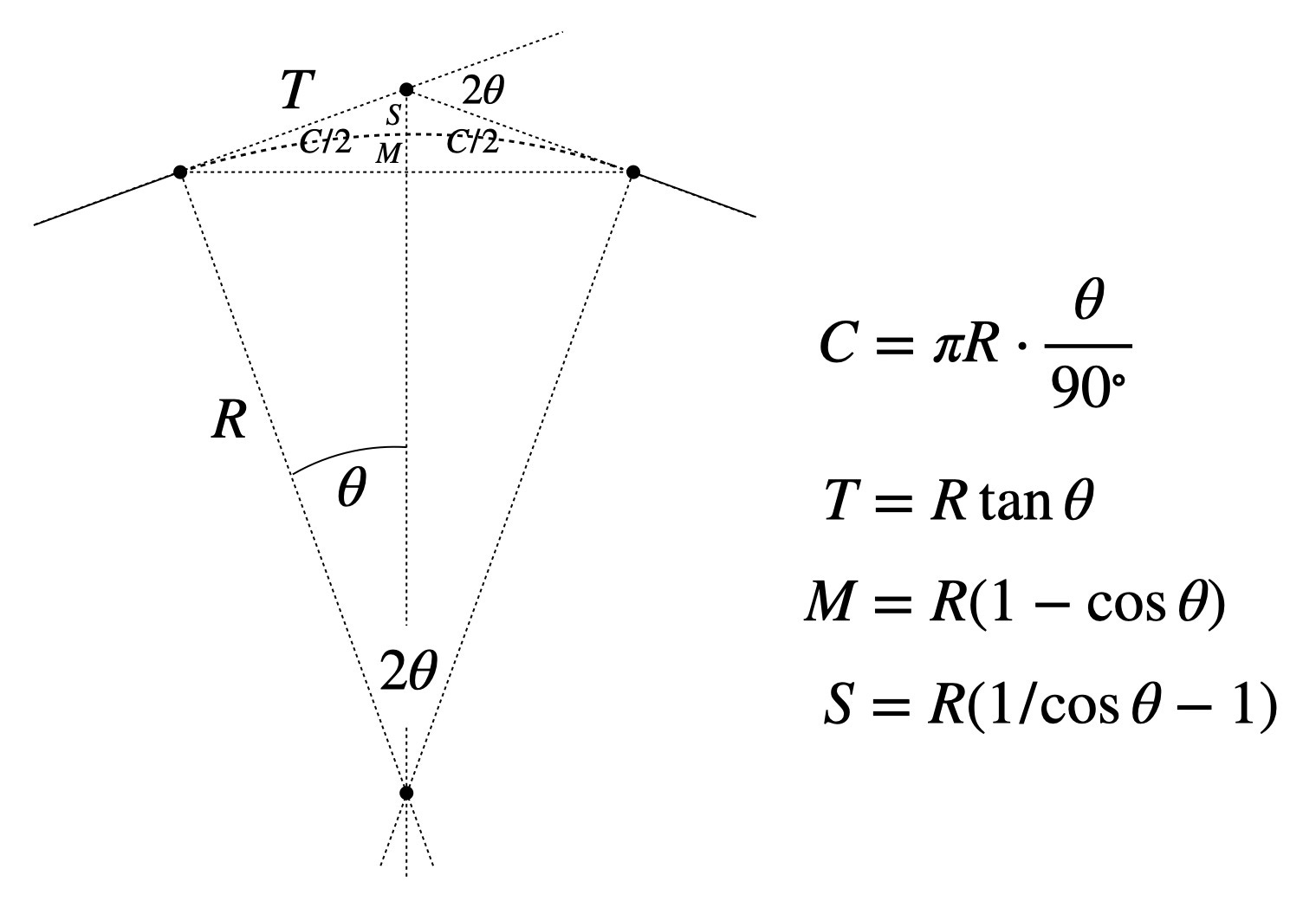
The length along the arc, C, is added to the list of relevant distances, as this is important for highway construction. And here, we use 𝜃 to denote the half-angle of the section of arc. Comparing these symbols to those used in the railroad case, 2𝜃 ⇿ I, and S ⇿ E. And next, I will explain why I’ve made the switch to new variable names.

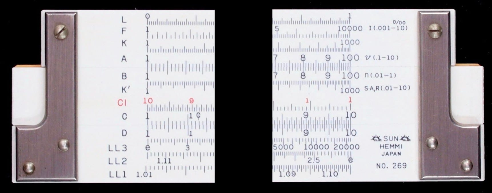
In 1965, Sun/Hemmi introduced their Hemmi Model 269 “Civil” duplex slide rule that included special scales with Civil Engineers in mind. As can be seen in the image below, the set of 26 scales includes the usual A/B, C/D, CI, DI, L, S, T, and so on, including three log-log scales. Interestingly, it has both a K scale on the body and another K scale — labeled K’ — on the slide. In addition, the slide rule also comes with stadia scales cos²𝜃 and sin𝜃cos𝜃 as well.

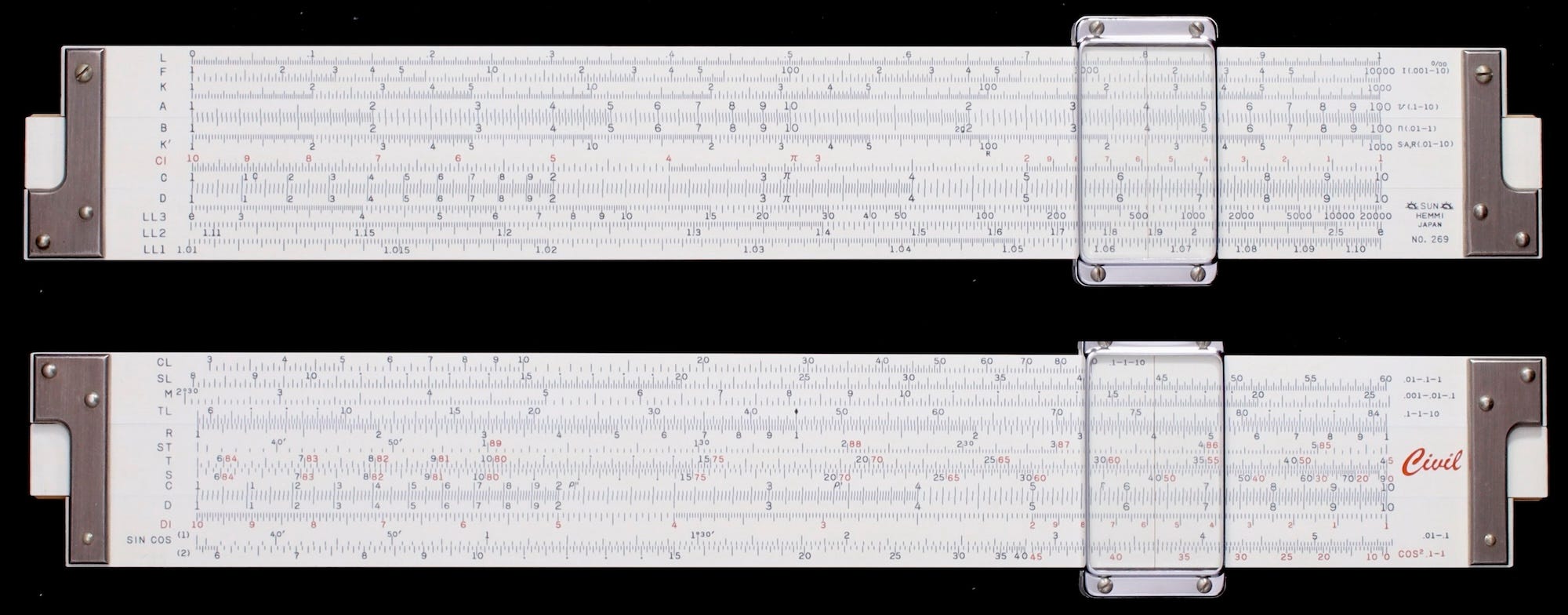
And then, there are 4 new scales: CL, SL, M, and TL. These provide calculations of the distances C, S, M, and T, respectively — emphasized in our new illustration above — for use in performing quick, direct curve calculations.

To illustrate the use of the “curve” scales, let’s perform the same calculation that was done for the railroad example earlier. From the example in the book, we had an arc of radius R = 925 ft, through a total angle I = 2𝜃 = 30^o 24’. The quantity E = R tanI/2 tanI/4 (= S) was calculated and found to be E = 33.5 ft, by finding two different angles, their tangents, multiplying them together, and multiplying by the radius R.

But now, this all can be performed in one step using the Hemmi 269. The angles used on the 4 new scales represent our “half-angle”, 𝜃. But to start things out, we set the value R = 925 ft on the R scale against the “diamond” symbol found on the TL scale. We then move the cursor to line up with our half-angle, 𝜃 = (30^o 24’)/2 = 15^o 12’, on the SL scale and read off the value of S. Note that all of the 4 new scales are marked in DMS (Degrees-Minutes-Seconds). On the R scale, we read the result, which I find to be about S = 33.2 ft, under the hairline.

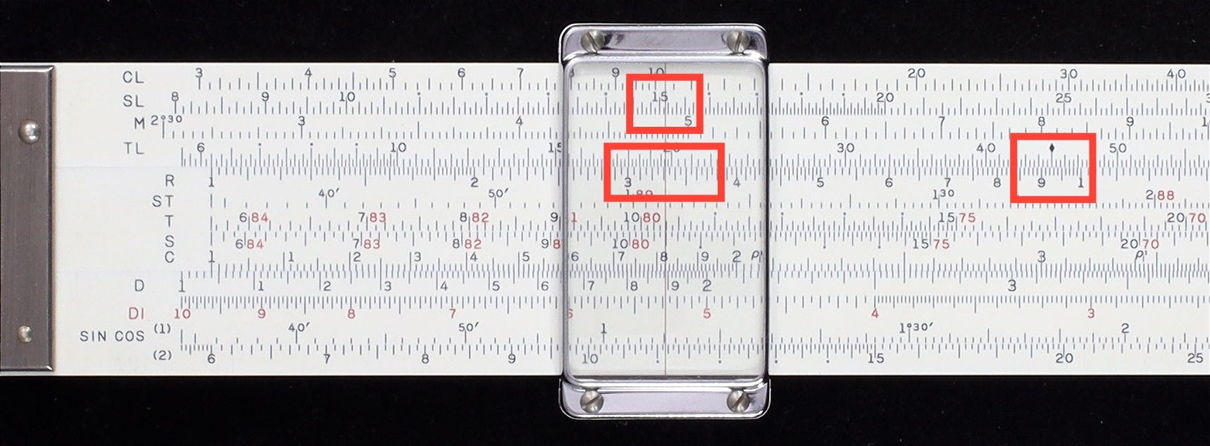
Without moving the slide (that is, the same setting of the radius R), moving the cursor to 15^o 12’ on the M scale, we find M = 32.4 ft; moving to 15^o 12’ on the CL we find C = 491 ft; and, moving to 15^o 12’ on the TL scale, we have T = 251 ft. All four calculations available in one setting of the slide. Quite the time saver!

To complete our description of the slide rule, it also offers one more scale, labeled F. This is a 4-decade logarithmic scale which, in conjunction with the K/K’ and A/B scales, can be used to perform water flow and drainage calculations as well, also important in civil construction. According to the manual that came with the rule, the equation being referred to is Manning’s Equation, used to find the velocity of flow in a conduit or culvert:

where v is the velocity of the fluid in m/s, A is the cross-sectional area of the fluid (in m²), S is the wetted perimeter of the conduit (in meters), R = A/S is the hydraulic radius, I is the hydraulic gradient or slope, and n is Manning’s coefficient, a constant with units of sec/m^1/3. The variable n depends upon the material, and has typical values from about 0.01 to 0.02 or so.

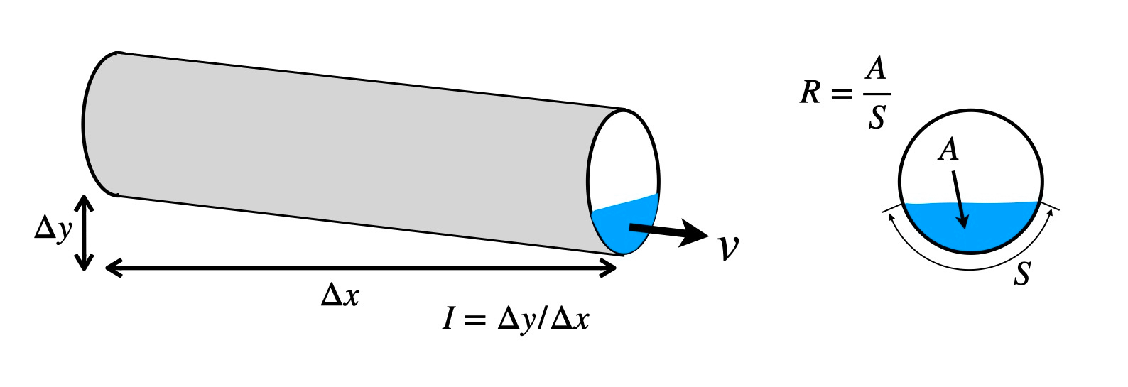
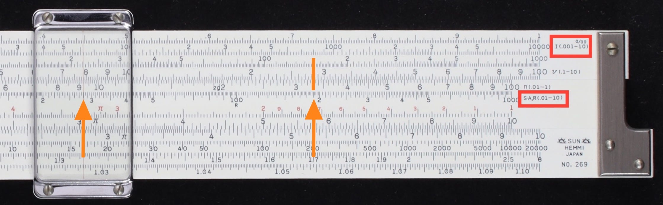
Let’s do a calculation. Suppose we have a 24-inch diameter pipe, flowing full. Then A = 𝜋 • 12² in² = 𝜋 • 0.3² m² = 0.28 m², S = 2𝜋 • 0.3 m = 1.9 m. We’ll use I = 0.08%, and n = 0.013, as taken from the 10-States Standards handbook.3 Note that each of the relevant scales has its limits shown on the right end for use in these calculations, with labels for the quantities provided. For example, the three decades of the K’ scale represent values of S from 0.01 to 0.1 to 1 to 10. Note, also, that the range of values on the F scale go from 0.01‰ to 10‰ (‰ = “per mil”, or per thousand); in terms of percent, the range of F is from 0.001% to 1%.

The standard calculation procedure is as follows: Placing the cursor at I on the F scale, move the slide to set S on the K’ scale at the cursor. Then, move the hairline to the value of A on the K’ scale. Next, moving the slide to bring n on the B scale to the hairline, one can read the velocity v on the A scale at the index of B. Using our numbers shown above, we find that v = 0.6 m/s.

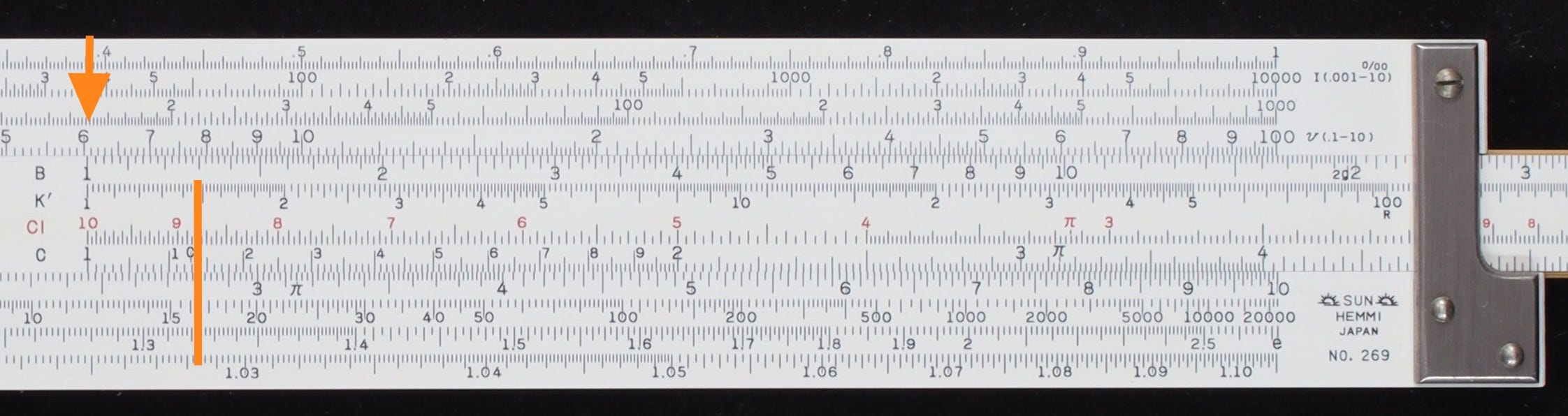
This calculation performed on the slide rule might be more easily viewed in the following way:

That is, we find A/S using K and K’. Since a number on F will be a number on K raised to the power of 4/3,4 we align I to multiply using the F scale. Then, with that result, the square root of a number on the F scale will appear on the A scale. The final division then can be performed using the B scale, with the final answer on A being located at the B index.

The manual also describes four other flow calculations that can be performed with the rule and its special arrangement of scales.

The Hemmi 269 is becoming one of my favorite slide rules. It has most of the basic scales anyone really needs, and the stadia scales and “curve” scales make a great set. And I’ve always thought more slide rules could have had a “K”-type scale on the slide to go along with the K scale on the body. The slide rule exhibits Hemmi’s famous bamboo construction, which makes it a pleasure to use, along with great precision in its scales. While the 269 is a specialty rule for civil construction, I find it to be a slide rule that could have gone well beyond that niche.

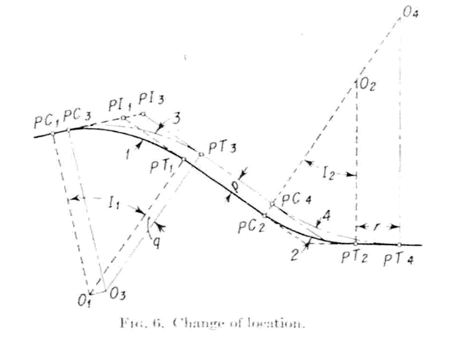
Civil construction of railways and highways is rich with computations of geometrical configurations, effects of gravity on performance (banked curves, water flow and drainage, etc.) and slide rules were used in all modern aspects of the trade, including special slide rules with special scales to improve accuracy and computational speed. Most projects do not involve just one or two arcs or curves, but actually quite many.

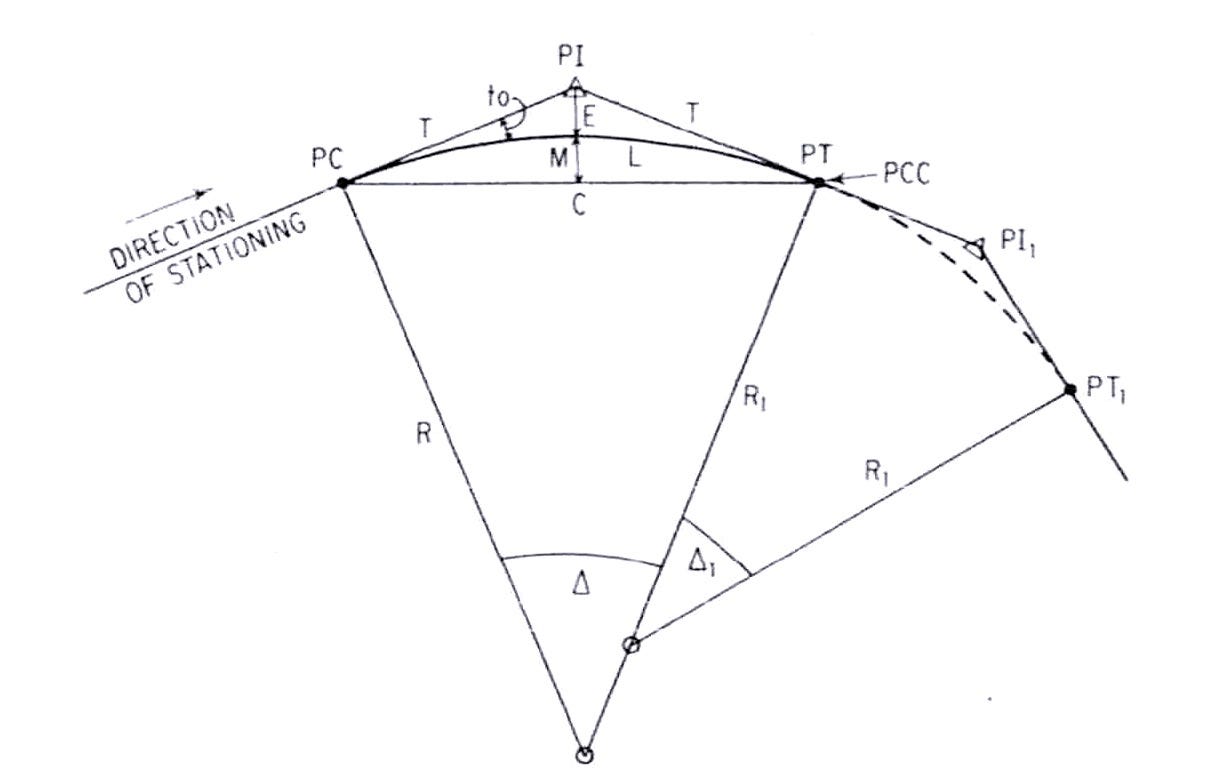
Computations can include not only design, but changes in surveying setup due to the constraints of the project terrain and other factors.

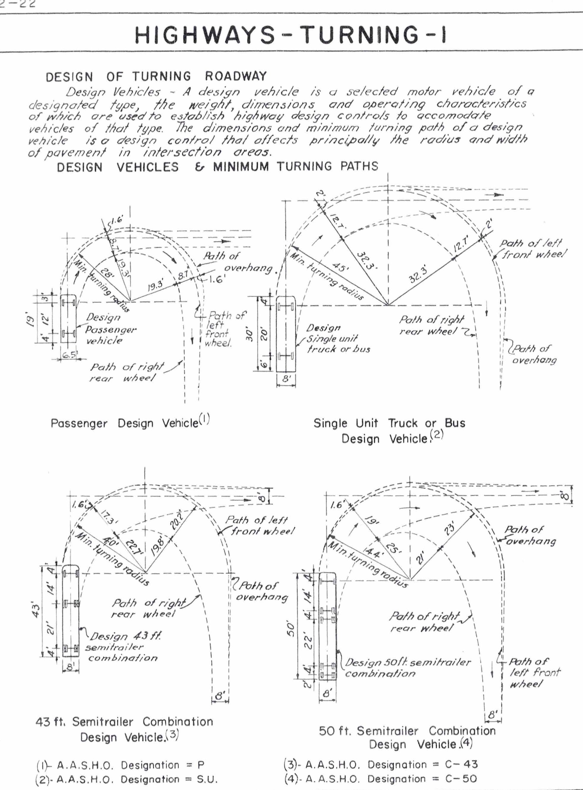
And highways have a range of vehicle sizes and shapes that need to be accommodated, leading to a variety of special arcs and curves.

Besides computing simple arcs and curves, we are all familiar with the banked curves on highways, the design of which relies on similar calculations as for the rail systems.

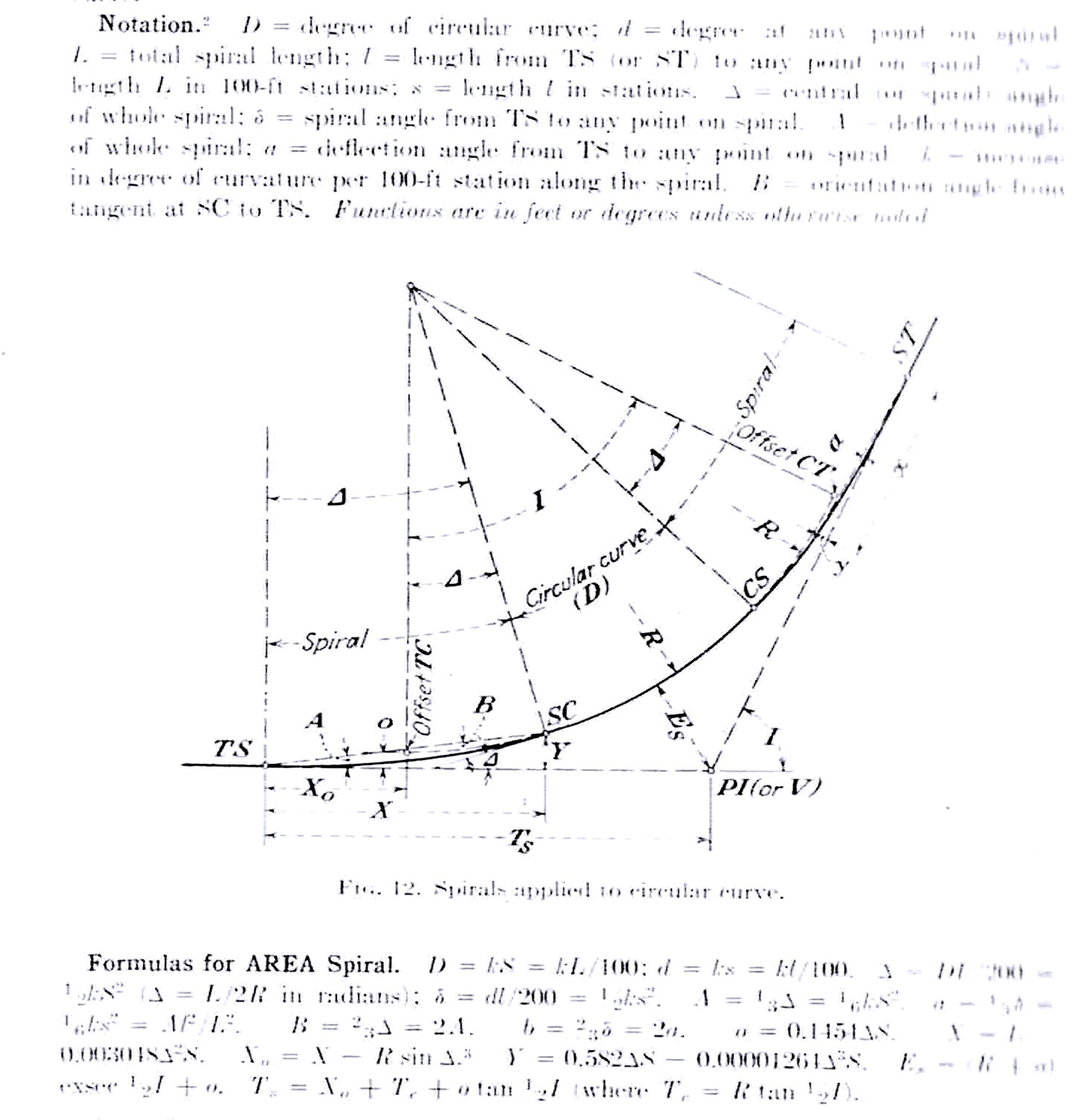
In this last image one can see the curve divided into “Spiral” sections on each end of a “Circular curve (D)”.

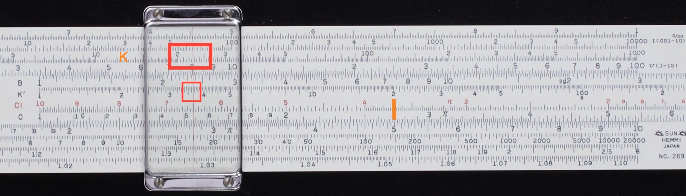
In fact, let’s re-do our calculation of l_e from the railroad discussion, but using our Hemmi 269 slide rule. The previous technique, using the standard Mannheim rule, took 3 cursor moves and 2 slide moves. To compute, using the Hemmi 269, the result of our equation l_c = S³D/2000,

• move the cursor to 5 (i.e., S = 50) on D. The cube of this number will be on K. Align “2” on K’ with the cursor, thus dividing by 2 (i.e., 2000). Move the cursor to 3.67 on K’, thus multiplying by D. Read 2.29 on K. From our earlier estimate of 250, the answer must be 229. Done — with two settings of the cursor, and only one setting of the slide.

And, just to “round things out”, here’s an image from Seelye’s book and his chapter on Railroads, written in 1996 (which could have been written in 1913):

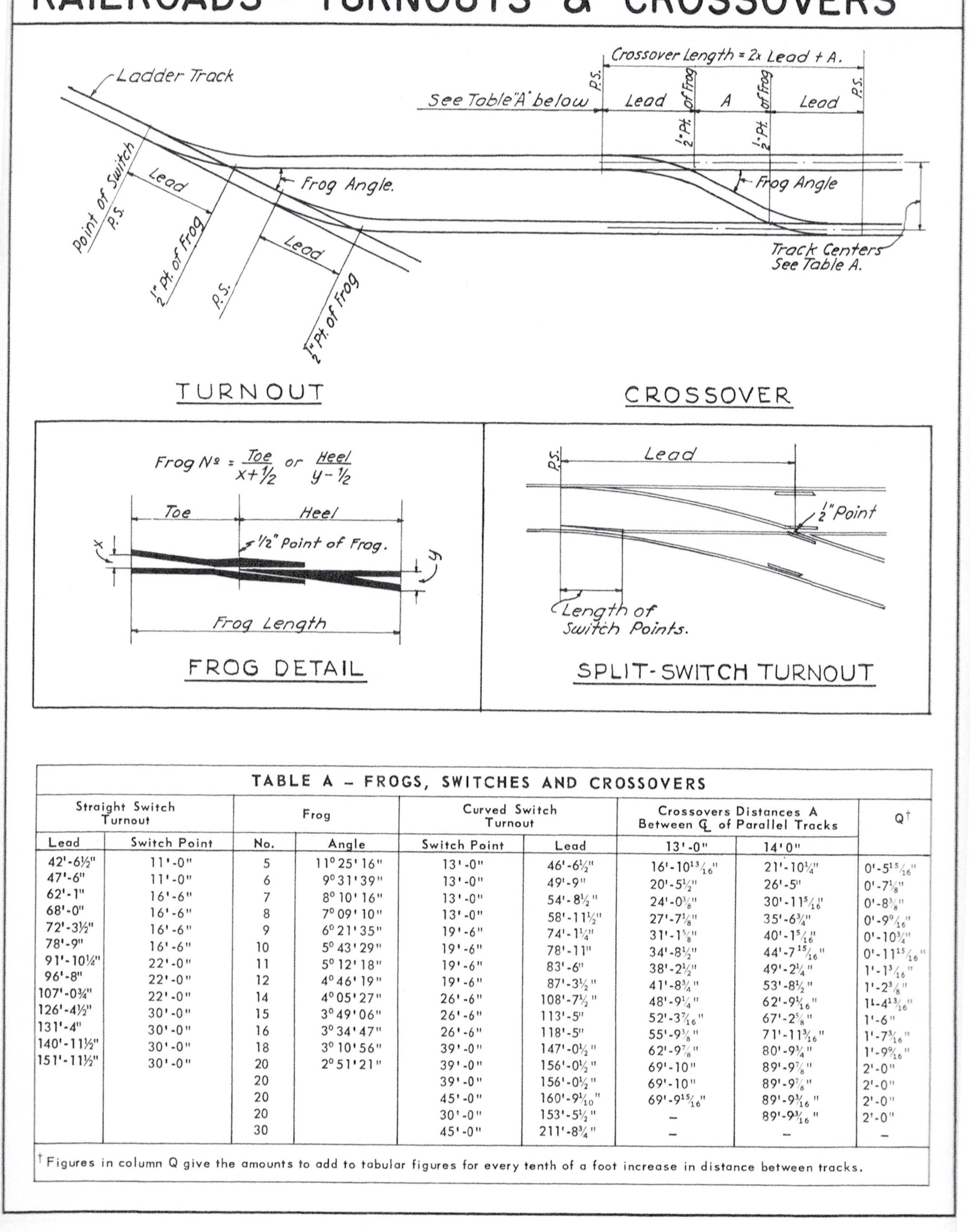
But what a difference a half-century makes. Having a slide rule that simplified the computation and layout of circular arcs in the field and other related problems must have been a very welcomed addition to the modern Civil Engineer’s “Box of Instruments.”

• Thomas Kentish, A Treatise on a Box of Instruments and the Slide-Rule, 2nd Edition, Relfe & Fletcher, London (1847).

• Arnold Jillson, Treatise on Instrumental Arithmetic, or Utility of the Slide Rule, The Case, Lockwood & Brainard Company, Hartford (1874).

• Fred T. Hodgson, The Mechanics’ Slide Rule, and How to Use It, The Industrial Publication Company, New York (1881).

• Charles N. Pickworth, The Slide Rule: A Practical Manual, Eighth Edition, D. Van Nostrand, Co., New York (1903).

• E.R. Cary, Solution of Railroad Problems by the Slide Rule, D. van Nostrand Co., New York (1913).

• John H. Perry and Robert H. Perry, Engineering Manual, McGraw-Hill, New York (1959).

• Leonard Church Urquhart, Civil Engineering Handbook, 4th Edition, McGraw-Hill, New York (1959).

• Frederick S. Merritt, Standard Handbook for Civil Engineers, McGraw-Hill, New York (1968).

• Tyler G. Hicks, Standard Handbook of Engineering Calculations, McGraw-Hill, New York (1972).

• Elwyn E. Seelye, Design, 3rd Edition, John Wiley & Sons, New York (1996).

I’d like to give special thanks to Kurt Dietrich for sharing with me excerpts from his books containing pertinent text on highway design and general engineering practices, and for giving me practical parameters to use in the “Manning” calculation.

Finally, speaking of trains, here’s a portion of my video of the Union Pacific 4014, the last remaining operational Union Pacific Big Boy — the world's largest operating steam locomotive (4-8-8-4 style, 600-ton, 133-foot-long, 7000 horsepower, built in 1941) — as we watched it pass through downtown Elburn, Illinois, just two months ago. (See this local CBS video for a nice overhead view.)