

If you are here, you already know that modeling the behavior of physical systems is often an exercise in solving Partial Differential Equations (PDEs).
A model PDE that applies to various problems is the diffusion equation. This is an incredibly common equation that is usually introduced from the perspective of heat conduction but it provides the underpinning for a large number of dynamical systems1.
The (linear) diffusion equation is given by
\(\partial_t T = \kappa \nabla^2 T\)
where T is a quantity that is defined in time and space, that is,
\(T=T(t,x)\)
For special initial conditions, T(t=0, x), the diffusion equation can be solved analytically to describe T(t, x).
This equation can also be solved numerically, but needs to be solved implicitly in time due to the severe CFL, time-step constraint. At Ergodic, we’re interested in differentiable numerical solvers so we will solve this using JAX.
Discretizing this system using backward differencing in time, and center differencing in space (BTCS), gives
\(\frac{T_i^{n+1}-T_i^n}{\Delta t} = \frac{\kappa_i^n}{\Delta x^2}\left(T^{n+1}_{i+1} - 2T^{n+1}_i + T^{n+1}_{i-1}\right).\)
This results in a tridiagonal system that can be directly inverted using the Thomas tridiagonal algorithm.
There is a budding ecosystem of tools to solve this problem using JAX. The two that we will use are diffrax and lineax. Diffrax is used to handle the time-stepping, and lineax has the tridiagonal solver.
We will specify the initial condition for the test problem. It is given by
\(T(t=0, x) =\frac{1}{\sqrt{\kappa a}} \exp\left(- \frac{x^2}{4 \kappa a}\right), \kappa = 0.1, a = 1000\)
The analytical solution to the diffusion equation with this initial condition is given by
\(T(t, x) = \frac{1}{\sqrt{\kappa (a+t)}} \exp\left(- \frac{x^2}{4 \kappa (a+t)}\right)\)
The numerical solution is also calculated. In the notebook, I show a calculation using a for loop and also using Diffrax. You’ll see that the Diffrax version is 10x faster.
This is what the solutions look like in comparison at t=800
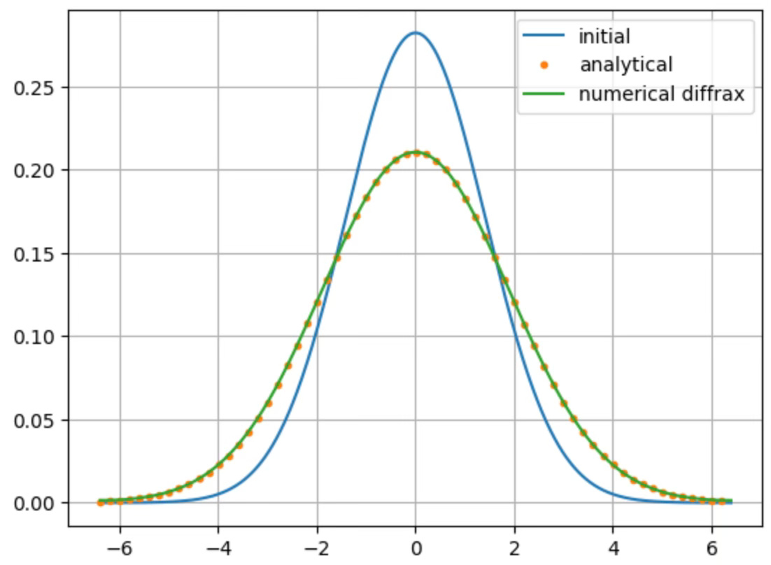
Seems like that worked. The error is less than 1% —
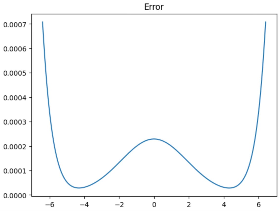
Not perfect, or even “high order” but good enough2
In more dimensions,
\(\partial_t T = \kappa \left(\partial_x^2 + \partial_y^2\right) T\)
The solution is slightly different
\(T(t, x, y) = \frac{1}{\kappa (a+t)} \exp\left(- \frac{x^2+y^2}{4 \kappa (a+t)}\right)\)
The discretization of the grid in space ends up resulting in a matrix that cannot be inverted directly.
\(\frac{T_{i, j}^{n+1}-T_{i, j}^n}{\Delta t} = \kappa_i^n\left(\frac{1}{\Delta x^2}\left(T^{n+1}_{i+1, j} - 2T^{n+1}_{i, j} + T^{n+1}_{i-1,j}\right) + \frac{1}{\Delta y^2}\left(T^{n+1}_{i, j+1} - 2T^{n+1}_{i, j} + T^{n+1}_{i, j-1}\right)\right).\)
One of the more popular ways of getting around this is using the Alternating Direction Implicit (ADI) scheme. In this scheme, you first perform half a time-step implicitly in 1 direction, half a time-step explicitly in the other direction, and then swap. That is,
explicit y for dt/2
implicit x for dt/2
explicit x for dt/2
implicit y for dt/2
This is directly solvable because you are only doing 1 dimensional diffusion solves. Miraculously, even though you do explicit diffusion solves, the solve remains stable.
The operator splitting ended up giving us
explicit solve for all x, y → trivially vectorized by just adding and multiplying arrays
implicit solve in x for each y → N_y linear solves
explicit solve for all x, y → trivially vectorized by just adding and multiplying arrays
implicit solve in y for each x → N_x linear solves
This is where you can leverage JAX’s vmap capability to solve N systems simultaneously. It composes with Lineax and is a very powerful operation that is easy to use. Here is what it looks like to map an “x solve” over all the y coordinates
linear_solve_x = vmap(partial(lx.linear_solve, solver=lx.Tridiagonal()), in_axes=(None, 1))Note the (None, 1). This lets us reuse the operator that is supplied at runtime across all y and only maps across axis=1 of the RHS array.
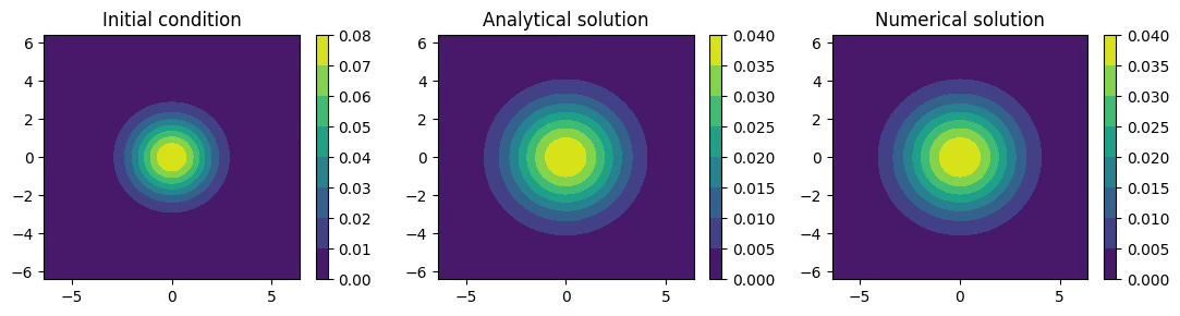
Looking pretty good!
Well, a diffusion solver by itself isn’t particularly exciting. But as I said at the beginning, a diffusion solve is an important component of most PDE solvers. For us, it is crucial for plasma physics applications. In fact, we use it inside ADEPT3 in various places and I was getting to the point where I needed a 2D version.
So in case you need one in JAX, like I did for differentiable plasma physics applications, here you go!
It should be easy to extend to 3D, and also to fix the boundaries. For enterprising young researchers, it could be an interesting project. Please submit a PR if you do take it on!
The code is provided at https://www.github.com/ergodicio/diffdiffusion
If you really zoom in and start thinking about the movement of each of the particles involved in this process, diffusion can become maddeningly complicated and leads to the concepts of entropy and irreversibility.
You could imagine the boundaries causing some problems eventually. There are ways to address this, namely by using a better linear system that handles the boundaries, and/or by using problem specific smoothers like taking the diffusion coefficient to 0 at the boundary because you know the quantity is negligible there anyway
https://github.com/ergodicio/adept
No posts
Comments
Nothing yet. Say the first thing.
Sign in to join the conversation.