The Hidden Tax of Memory in Model Inference

A few days ago, I was sitting around letting my agents cook in Cursor when I started paying attention to the little status messages flashing across the screen: “Planning next steps.” “Thinking.” “Contemplating.”

Very calm. Very sophisticated. Almost peaceful.

Meanwhile, underneath that tiny word “thinking,” an absolutely deranged amount of machinery was springing into action. Billions of numbers were being pulled through memory, multiplied together, passed between chips and slowly turned into the next token.

That gap is what got me interested. We’ve made interacting with these models feel unbelievably simple. You type something, the model “thinks,” and words appear. But producing those words requires one of the most complicated and expensive computing systems humans have ever built.

And a surprisingly large part of that complexity comes down to one basic problem: the model is enormous, and all those numbers need somewhere to live.

At the simplest possible level, an AI model is an enormous collection of numbers.

Those numbers are called parameters, and they contain the patterns the model learned during training. A 70-billion-parameter model contains roughly 70 billion of them. It’s basically a spreadsheet from hell.

When you ask the model a question, a processor uses those numbers to calculate what should come next. Then it does it again for the next token. And again. And again.

But the numbers have to be stored somewhere the processor can reach them quickly. The larger the model gets, the more numbers it contains and the more memory it needs.

That’s the whole problem in its simplest form:

Big models contain lots of numbers. Lots of numbers need lots of memory. And fast memory is painfully expensive.

A parameter is often described as a tiny adjustable knob inside the model.

At the beginning of training, most of these knobs contain fairly useless values. The model reads some text, tries to predict what comes next and compares its answer with what actually came next. When it gets the answer wrong, training nudges billions of those knobs slightly.

Then it does that again.

And again.

And again, an absolutely disgusting number of times.

Eventually, the values stop being random. Together, they begin to capture relationships in the training data. The model learns that certain words tend to appear together, that code follows particular structures, that Paris is associated with France and that putting rm -rf into the terminal might make your afternoon significantly worse.

It’s important not to take the knob analogy too literally. There usually isn’t one parameter containing “Paris” and another containing “France.” Knowledge is spread across enormous groups of parameters and represented through the relationships between them.

Underneath everything, those parameters are organized into giant grids of numbers called tensors. Most of the work performed by an LLM involves taking data, passing it through these tensors and multiplying an ungodly number of values together.

The code tells the computer how those operations should happen. The weights contain the values the model learned.

That distinction matters. The actual inference engine might only be a relatively small piece of software. The model weights can be hundreds of gigabytes or even several terabytes.

You can see this yourself in Llama 3.1 70B’s file repository. Scroll past the small configuration and tokenizer files until you reach the giant numbered files ending in .safetensors.

Those files are chunks of the model’s learned weights. They’re split into multiple pieces because the full collection is too large and annoying to handle as one enormous file. When you load the model through Hugging Face, those chunks are reassembled into the tensors used during inference.

So when you download a model, you’re not downloading a giant database of sentences or a compressed copy of the internet. You’re downloading billions of learned numerical relationships.

And before the processor can use those relationships, every one of those numbers needs a physical representation in memory.

That brings us to the next problem: how many bytes does a billion numbers actually require?

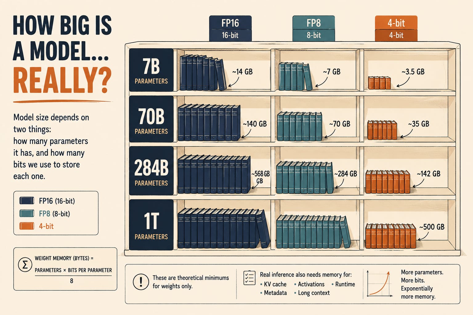
Knowing that a model contains 70 billion numbers is only half the story. The other half is how much space we use to store each one.

Computers store numbers as bits. The more bits we give each parameter, the more precisely we can represent its value. More precision can preserve more information, but it also makes the model much larger.

The basic math is refreshingly simple:

We divide by eight because there are eight bits in a byte.

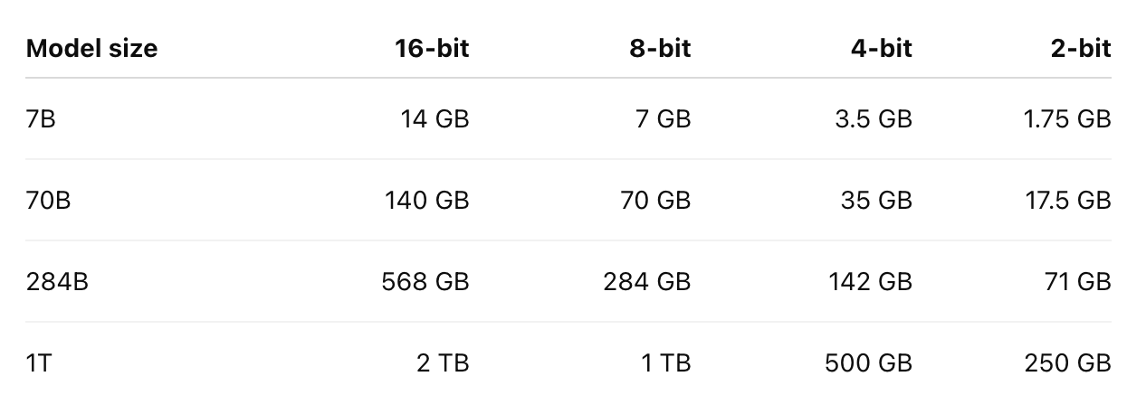
Let’s take a 70-billion-parameter model:

• At 16 bits per parameter, it needs roughly 140 GB.

• At 8 bits per parameter, it needs roughly 70 GB.

• At 4 bits per parameter, it needs roughly 35 GB.

• At 2 bits per parameter, it theoretically needs roughly 17.5 GB.

Same number of parameters. Wildly different amount of memory.

This process of storing parameters with fewer bits is called quantization.

The easiest way to think about quantization is rounding. Imagine the original model wants to store a value like 0.738194. A lower-precision version might store something closer to 0.74, 0.75 or even 0.5, depending on how aggressive the quantization is (this isn’t exactly how quantization works, but it’s a post for another day).

Do that once and it barely matters. Do it across 70 billion parameters and you can shrink the model dramatically.

Of course, there’s no free lunch. Use too few bits, round the values too aggressively and the model can start losing accuracy. The art of good quantization is finding a much smaller representation without making the model noticeably dumber.

You can watch this tradeoff happen in the real world. This quantized 70-billion-parameter DeepSeek repository offers versions ranging from about 15.9 GB to 50 GB. They all come from the same underlying model, but they use different GGUF quantization formats to decide how much precision to preserve.

The simple table above is only the starting point. Real quantized models also need scales, metadata and sometimes different precisions for different parts of the network. That’s why an actual 4-bit model might not land at exactly four bits per parameter.

But the big idea holds:

The number of parameters tells you how many numbers the model contains. The precision tells you how much space each number occupies.

Quantization can make the model dramatically smaller. It can turn a model that needs several expensive accelerators into one that fits on a single machine.

But “fits on a machine” still leaves us with an important question.

Fits where?

Let’s say you download a 42 GB quantized model onto a computer with a 1 TB SSD and 32 GB of RAM. The download worsks perfectly. You’ve got plenty of storage, the model is sitting right there and everything seems fine.

Then you try to run it, and your computer starts wheezing.

The problem is that your 1 TB SSD doesn’t give you 1 TB of working memory. It gives you a large place to store files when you aren’t actively using them. The processor can’t work with those files nearly as quickly as it can work with data sitting in RAM.

The easiest way to picture this is with a desk and a warehouse:

• The SSD is the warehouse. It’s big, cheap and great for storing an enormous collection of books.

• RAM is the desk. It’s smaller and more expensive, but everything placed there is much easier to reach.

• The model weights are the books. They contain the information the processor needs to do its work.

• The processor is the person at the desk. It’s trying to read those books quickly enough to answer your question.

If all the books fit on the desk, the processor can keep reading and working. If the model is 42 GB and you’ve only got 32 GB of RAM, some of those books have to stay in the warehouse.

That doesn’t always mean the model can’t run. The computer has a few options:

• Refuse to load the model.

• Keep only part of the model in memory.

• Fetch different pieces from the SSD as they’re needed.

• Split the model across several devices.

The last three can all work, but none of them is free. If the processor has to stop and wait for another chunk of the model to arrive, it isn’t spending that time generating tokens. It’s also coordinating a deeply annoying book-delivery service.

This is why a computer with several terabytes of storage can still struggle to run a model that’s only a few dozen gigabytes. The model fits on the computer. It just doesn’t fit where the computer needs it.

Where the weights need to live depends on the hardware:

• A CPU usually works with weights stored in system RAM.

• A discrete GPU usually works with weights stored in its own VRAM.

• A high-end AI accelerator normally uses an extremely fast and expensive form of memory called HBM.

• An integrated system may let the CPU and GPU share one larger pool of unified memory.

We’ll get into each of those shortly. For now, you only need to know that the processor wants the model’s weights close by, and moving them from one place to another takes time.

That’s why tools for loading very large models spend so much effort deciding which parts should live on which device. They aren’t just opening a file. They’re trying to place billions of numbers somewhere the processors can reach without constantly stopping to wait.

There are clever ways to run models that don’t completely fit in memory. You can leave some weights on an SSD, move layers around while the model runs or split the model across several pieces of hardware.

But none of those tricks makes the memory problem disappear. They just make a trade:

The model fits, but now it has to commute.

And as anyone who’s ever lived in Los Angeles knows, commuting can ruin everything.

Let’s go back to that little “thinking” message in Cursor.

It feels like the model reads your request, thinks about the answer and then writes a response. That’s a useful illusion, but it isn’t really what’s happening.

A language model generates text one token at a time.

A token can be a word, part of a word, a number, a punctuation mark or even a bit of whitespace. You can play with OpenAI’s tokenizer to see how normal text gets chopped into these smaller pieces.

The sentence:

The model needs somewhere to live.

might be split into pieces that look something like:

The model needs somewhere to live .

The exact split depends on the tokenizer, but the basic process is always the same. The model isn’t generating an entire sentence in one shot. It’s repeatedly answering one question:

Given everything I’ve seen so far, what token should come next?

To answer that question, the model goes through a simplified process:

1. Your prompt gets split into tokens.

   The model doesn’t read raw text directly. The tokenizer converts your words into a sequence of token IDs.

2. Those token IDs become vectors.

   Each token gets turned into a collection of numbers the model can work with. These are called embeddings.

3. The vectors pass through the model’s layers.

   Every layer transforms those numbers. As the data moves deeper into the model, it builds a richer representation of what the prompt means and what should come next.

4. The model produces probabilities for the next token.

   It doesn’t immediately output one perfect answer. It assigns probabilities to thousands of possible tokens.

5. One token gets selected.

   Depending on the model’s settings, it might choose the most likely token or sample from several likely options.

6. The selected token gets added to the sequence.

   Then the model runs the process again to generate the token after that.

And again.

And again.

And again, until the response is finished or the agent decides it would rather spend another five minutes “contemplating.”

If you want the much more detailed version, Jay Alammar’s Illustrated Transformer is still one of the best visual explanations of what’s happening inside these layers.

For our purposes, the important thing is that every generated token has to travel through the model.

Think of the model as a giant factory. Each layer is another station on the assembly line. A token enters the factory, passes through every station and eventually comes out as a prediction for what should happen next.

Then the next token enters the factory.

The model’s weights normally stay loaded in memory throughout this process. They aren’t being downloaded from the SSD again for every token. But the processor still has to read and use those weights every time information passes through the model.

That distinction matters.

The model might only be loaded into memory once, but its weights get used over and over again. For a normal dense model, nearly every layer participates in generating every new token.

A 70-billion-parameter model doesn’t become a small model after it produces the first word. It’s still a 70-billion-parameter model for the second word, the third word and the awkwardly long explanation it produces after ignoring your request to “keep it short.”

First, the weights have to fit in memory.

Then memory has to deliver them fast enough.

Memory capacity tells us whether the model fits.

Memory bandwidth tells us how quickly the processor can read it.

Those sound like similar problems, but they’re very different.

Imagine two desks that can each hold every book in our enormous model library. One desk has an assistant who can deliver 100 pages per second. The other has an assistant who can deliver 1,000 pages per second.

Both desks have enough capacity. But the person at the second desk can work much faster because they spend less time waiting for pages.

That’s memory bandwidth.

It measures how much data can move between memory and the processor every second. If the processor can perform calculations faster than memory can supply the weights, the processor sits around waiting.

This happens a lot during LLM inference because modern GPUs are outrageously good at math. The harder part is continuously feeding them enough data to keep all that math hardware busy.

There are actually two different phases of inference:

• Prefill happens when the model first reads your prompt. It can process many prompt tokens together, which creates a lot of work for the processor and often makes better use of the GPU’s compute.

• Decode happens after that, when the model generates the response one token at a time. Each step performs a smaller amount of work while still needing access to the model’s weights.

That second phase is where memory bandwidth often starts dominating.

A very simplified way to think about the limit is:

This isn’t a perfect benchmark formula. Real performance also depends on batching, attention, cache size, kernels, quantization, communication and roughly a thousand other engineering details designed to make benchmarking arguments on the internet unbearable.

But it captures the main idea.

Suppose a model needs to read roughly 100 GB of active weights to generate each token. If the memory system can deliver 1 TB per second, the absolute best-case mental model gives you around ten tokens per second for one sequence.

Give the processor twice as much raw compute but the same memory bandwidth, and it may not get much faster. It was already waiting for memory.

Give it twice the memory bandwidth, and now it can feed those compute units more quickly.

Batching can improve the equation. If several users are generating tokens at the same time, the system can load a chunk of weights and use it across multiple sequences. That lets it perform more useful math for each byte pulled from memory.

But batching doesn’t make bandwidth irrelevant. It changes how efficiently you use it.

This is why two machines that can both fit the same model may generate tokens at completely different speeds. The important question isn’t only:

Does the model fit?

It’s also:

How quickly can the hardware drag all those numbers past the processor?

Everything we’ve discussed so far describes a dense model.

In a dense model, nearly all the model’s layers and weights participate in generating every token. If it’s a 70-billion-parameter dense model, you’re broadly doing work across those 70 billion parameters each time information passes through it.

Many of the largest modern models use a different design called Mixture of Experts, or MoE.

Instead of using the same giant block of weights for every token, an MoE model contains lots of smaller specialist networks called experts. A router looks at each token and decides which experts should handle it.

Think of it like an enormous consulting firm.

The firm might employ hundreds of specialists, but you don’t invite every employee to every meeting. You look at the problem and pull in the handful of people who might actually be useful.

An MoE model works in roughly the same way. When a token reaches an MoE layer, a router scores the available experts, selects a small group and sends the token through them. Their results get combined, and the token moves onward.

Hugging Face describes this process in its experts interface documentation: for each token, a router selects a small number of experts and runs the token through their parameters.

This gives an MoE model two different parameter counts:

• Total parameters tell you how many parameters exist across the full model.

• Active parameters tell you roughly how many participate in processing one token.

DeepSeek-V3 is a great example. It contains 671 billion total parameters, but only about 37 billion are activated for each token. In its routed MoE layers, it has 256 routed experts and selects eight of them for each token, according to the DeepSeek-V3 technical report.

That makes each token much cheaper to calculate. Instead of pushing every token through all 671 billion parameters, DeepSeek only uses a much smaller slice of the model.

This is great for compute.

It doesn’t mean you only need enough memory for 37 billion parameters.

The first token might need one group of experts. The next token might need another. A different user’s request could produce a completely different routing pattern.

You don’t know exactly which experts will be selected until the router sees the token. That means every expert still needs to be available somewhere.

At a rough theoretical minimum, DeepSeek-V3’s 671 billion total parameters would require approximately:

• 1.34 TB at 16-bit precision

• 671 GB at 8-bit precision

• 336 GB at 4-bit precision

And that’s only for the model weights. The real system also needs memory for the KV cache, temporary activations, routing, quantization metadata and enough breathing room to serve actual users.

The 37 billion active parameters reduce how much data and computation a particular token needs. They don’t magically shrink the complete model from 671 billion parameters to 37 billion.

So where do the other 634 billion parameters go?

You’ve basically got three options:

• Keep the entire model in one enormous pool of memory.

• Split the experts across several GPUs or machines.

• Leave some experts on an SSD and load them when the router selects them.

The first option is simple but expensive. You need a machine with hundreds of gigabytes, or potentially terabytes, of fast memory.

The second option is how many large MoE models are actually served. Each device keeps a subset of experts in its own memory. One GPU might hold experts 1 through 32, while another holds experts 33 through 64.

Taken together, the cluster still needs enough RAM or HBM to hold the entire model. MoE changes where the weights live. It doesn’t remove them.

The third option saves memory, but it can make inference painfully slow. If the router selects an expert sitting on an SSD, the system has to load those weights before it can continue generating the token.

The model technically fits.

Unfortunately, some of its employees are commuting to every meeting from a warehouse.

You can make this smarter by keeping popular experts in memory, predicting what might be needed next or loading experts before the router reaches them. But routing changes across tokens and users, so the system can’t always know what’s coming.

This is why MoE reduces the compute and bandwidth tax without eliminating the capacity tax.

The active parameters tell you how much of the consulting firm attends one meeting.

The total parameters tell you how much office space the company still needs.

MoE lets you avoid asking all 671 billion employees to speak at once. It doesn’t let you fire the other 634 billion or store them in a closet without consequences.

At this point, there’s an obvious question.

If an MoE model only uses a handful of experts for each token, why do we need to keep every expert in expensive memory? Why not leave the inactive ones on an SSD and load them into RAM or HBM only when the router selects them?

You absolutely can.

Researchers and inference engines are actively working on expert offloading, expert caching and predictive loading. The problem is that you’re swapping a memory-capacity problem for a data-movement problem.

And inference really, really hates waiting for data.

Imagine the router decides that the next token needs experts 17, 42, 88 and 201. If those experts are already sitting in HBM, the GPU can start using them almost immediately.

If expert 88 is sitting on an SSD, the system has to:

1. Read the expert’s weights from storage.

2. Move them into system RAM.

3. Copy them across the PCIe connection into the GPU’s HBM.

4. Wait until the transfer finishes.

5. Run the expert.

6. Potentially evict it again to make room for whatever the next token needs.

That’s a lot of shuffling just to generate part of one token.

The speed difference between these memory tiers is enormous. A fast consumer NVMe SSD might read sequential data at around 7 GB per second. An H100’s HBM can deliver several terabytes per second.

Those numbers aren’t perfectly comparable because real transfers depend on access patterns, software and hardware. But they show the basic problem. HBM can feed a GPU hundreds of times faster than a single SSD can feed it.

There’s also latency. SSDs are great at moving large, orderly streams of data. MoE routing can produce lots of smaller, unpredictable requests scattered across different experts. That’s a much uglier workload.

The router can select different experts:

• At every MoE layer

• For every token

• Across every request in a batch

• As the conversation and generated response change

So this isn’t like loading one model at startup and leaving it alone. The working set can keep changing while the model is running.

If the required expert isn’t already in fast memory, you get a cache miss. The GPU then has to wait while the expert travels up the memory hierarchy.

That path might look like this:

SSD → system RAM → GPU HBM → computation

Technologies like NVIDIA GPU Direct Storage can remove the stop in system RAM and move data more directly from storage to GPU memory. That helps, but it doesn’t turn an SSD into HBM. You’ve shortened the commute. You haven’t moved the warehouse next door.

The obvious solution is to keep the most popular experts in memory and leave the rarely used ones on storage. That works when expert usage is predictable and the cache hit rate stays high.

But popular experts can change with the workload. A coding request, a translation request and a chemistry question might all activate very different parts of the model. Add thousands of users asking unrelated questions, and your nice orderly expert cache can turn into musical chairs.

Batching makes this even harder. One user’s token might need four experts while another user’s token needs four completely different ones. Across a large batch, the supposedly sparse model may touch a surprisingly large portion of its experts.

You can try to predict the next experts and begin loading them early. Researchers have built systems that do exactly that. But now your serving stack needs another prediction system whose job is to guess what the prediction system will need next.

AI infrastructure is nothing if not committed to the bit.

If the prediction is right, you can hide some of the transfer behind other computation. If it’s wrong, you’ve wasted bandwidth loading an expert you didn’t need, and you may still have to stop for the one you missed.

So SSD offloading has a real place:

• It can make an otherwise impossible model fit on cheaper hardware.

• It can work well for experiments and low-throughput local inference.

• It can help when expert routing is predictable.

• It can reduce the amount of expensive RAM or HBM you need.

What it usually can’t do is match the latency and throughput of keeping the model resident in fast memory.

One recent on-demand MoE loading system managed to use roughly one-third of the GPU memory while retaining about 75% of the decoding speed of a fully cached deployment. That’s genuinely impressive. It’s also a nice demonstration of the trade. The memory savings were real, but they weren’t free.

This is the central tension with expert offloading:

Storage makes enormous models possible. Memory makes them fast.

Keeping inactive experts on an SSD lets you avoid paying the entire memory bill upfront. But every cache miss sends part of that bill back to you as latency, lost throughput and extra system complexity.

The experts don’t need permanent desks in HBM.

They do, however, need to show up for work incredibly quickly.

We’ve already seen one version of this problem with MoE models. You can leave inactive experts on an SSD and load them only when the router asks for them, but every cache miss forces the system to move weights from slow storage into faster memory. The model fits, but it also spends a depressing amount of time commuting.

That same tradeoff applies to the rest of the model. Once the weights no longer fit in the memory attached to one processor, you’ve got a few options:

• Keep some weights in system RAM.

• Leave some weights on an SSD.

• Split the model across several GPUs.

• Place different MoE experts on different devices.

• Quantize the model until it squeezes into the hardware you already own.

All of these approaches work. The question is what you’re willing to sacrifice in return. You can trade memory for slower transfers, buy more hardware or accept the communication overhead that comes with turning several computers into one giant virtual machine.

The memory bill never disappears. It just shows up somewhere else.

Let’s say you’ve got a 70 GB model, a GPU with 48 GB of HBM and a machine with 128 GB of ordinary system RAM. The model can’t fit entirely on the GPU, but it can fit comfortably in the machine’s combined memory.

CPU offloading lets you keep some weights in system RAM and move them onto the GPU when they’re needed. Hugging Face’s CPU offloading tools can store the weights in CPU memory, transfer each section onto the GPU for its calculation and then remove it again to make space for the next one.

In practice, the process looks roughly like this:

1. Find the next layer’s weights in system RAM.

2. Copy those weights across PCIe.

3. Place them in the GPU’s HBM.

4. Run the layer.

5. Remove the weights if the space is needed elsewhere.

6. Repeat with the next layer.

That’s still much faster than fetching weights from an SSD, but system RAM and GPU HBM aren’t the same thing. HBM sits next to the GPU and is built to feed it enormous amounts of data. System RAM usually lives on the other side of the CPU and has to send data across PCIe before the GPU can use it.

The system can hide some of that delay by moving the next layer while the GPU processes the current one. If the transfer finishes in time, the GPU keeps working without much interruption. If it doesn’t, the GPU stalls while it waits for its next delivery.

This creates a slightly absurd situation where an incredibly powerful GPU can spend part of its time doing absolutely nothing. It has plenty of computational power. It just doesn’t have the numbers it needs yet.

CPU offloading can still be a great option when you’re experimenting locally, serving a small number of requests or trying to run a model that would otherwise require another GPU. It saves expensive HBM capacity and replaces it with cheaper system RAM.

But that savings comes with a toll. The more weights you move between RAM and HBM, the more inference performance depends on the connection between them.

We’ve already covered SSD offloading in the context of inactive MoE experts. The same technique can be applied to ordinary model layers when the full model doesn’t fit in GPU memory or system RAM.

Hugging Face supports disk offloading for exactly this situation. Some weights can remain as memory-mapped files on storage, and the system reads them into faster memory as the model reaches them.

The normal path looks something like:

SSD → system RAM → GPU HBM

Technologies like NVIDIA GPU Direct Storage can shorten that route by moving data more directly from storage into GPU memory. That removes an unnecessary stop, but it doesn’t turn an SSD into HBM. You’ve built a better highway from the warehouse. The warehouse is still nowhere near the desk.

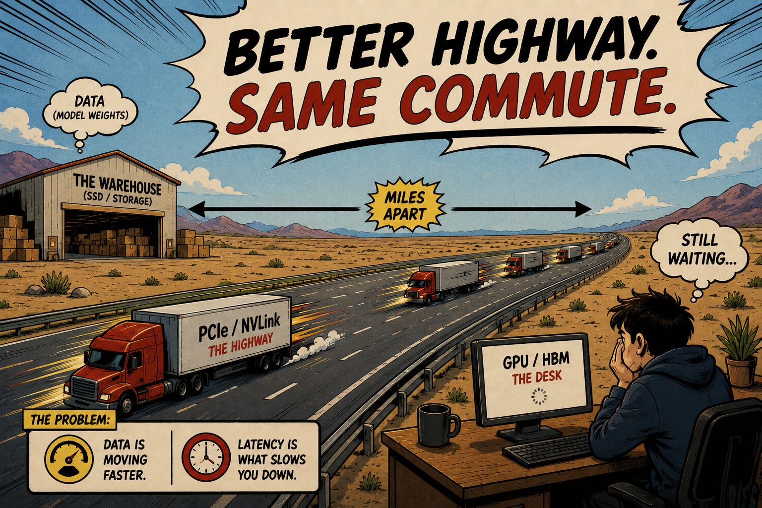
A modern SSD might read large sequential files at several gigabytes per second. Modern HBM can move several terabytes per second. Those aren’t perfectly comparable numbers, and real performance depends on the exact hardware and access pattern, but the size of the gap tells you why SSD offloading hurts.

The software can make this less painful in a few ways:

• Memory mapping loads only the file pages that are currently needed.

• Prefetching begins loading the next weights before the processor reaches them.

• Caching keeps frequently accessed weights in RAM or HBM.

• Pinned memory can make transfers from system RAM to the GPU more efficient.

• Direct storage access can avoid extra copies through the CPU.

These techniques can turn an impossible deployment into a functional one. They’re especially useful for experimentation, low-volume inference or workloads where waiting longer is acceptable.

But “the model runs” doesn’t mean “the model serves efficiently.” If different layers or experts have to be loaded repeatedly from storage, token generation starts pausing around those transfers. Under concurrent traffic, different requests may also need different parts of the model, making the cache less predictable and the latency more chaotic.

That’s why production providers usually prefer to keep frequently used weights in RAM or HBM. An SSD gives you enormous capacity at a reasonable price. It doesn’t give you the speed or predictability required to serve lots of users without making them stare at a blinking cursor.

The more common production solution is to stop trying to force the entire model onto one GPU. Instead, you divide it across several GPUs and use their combined memory.

Imagine a 280 GB model and four GPUs with 80 GB of HBM each. After reserving room for the KV cache and other runtime state, no individual GPU can hold the model. Together, the four GPUs have enough capacity.

There are two common ways to divide the model: pipeline parallelism and tensor parallelism.

Pipeline parallelism splits the model by layer. A simplified 80-layer model might be divided like this:

• GPU 1: Layers 1 through 20

• GPU 2: Layers 21 through 40

• GPU 3: Layers 41 through 60

• GPU 4: Layers 61 through 80

The input begins on GPU 1. Once that GPU finishes its layers, it sends the intermediate result to GPU 2. The result continues down the line until it reaches the final stage and becomes the next token.

DeepSpeed describes pipeline parallelism as partitioning a model into stages that live on different devices. Each GPU stores only its own portion of the weights, so the full model no longer has to fit on one device.

The downside is that the GPUs depend on one another. GPU 4 can’t complete the token until GPUs 1, 2 and 3 have performed their parts. With only one request moving through the system, some GPUs may sit idle while they wait for work to arrive. This unused time is called a pipeline bubble.

You can reduce those bubbles by processing several requests at once. While GPU 2 works on one request, GPU 1 can begin processing another. This improves the total throughput of the cluster, although it doesn’t necessarily make one individual request much faster.

Pipeline parallelism solves the memory problem by turning the model into an assembly line. The assembly line works best when there’s enough traffic to keep every station busy.

Tensor parallelism cuts the model in a different direction. Instead of assigning entire layers to different GPUs, it splits the large tensors inside each layer.

Each GPU stores and calculates one portion of the same matrix. The GPUs then exchange and combine their partial results before moving into the next operation. DeepSpeed’s tensor-parallel inference tools automate this for supported model architectures.

A simplified layer might work like this:

1. Each GPU reads its local shard of the weights.

2. Each GPU calculates a partial result.

3. The GPUs exchange or combine those results.

4. The completed output moves into the next operation.

5. The process repeats throughout the model.

This lets several GPUs work on the same layer at once, which can reduce latency as well as memory per device. But the GPUs now need to communicate constantly. A model with dozens of layers may require many synchronization operations while generating a single token.

Fast connections like NVLink can make that manageable. Slower links can turn communication into the new bottleneck. The GPUs finish their local calculations and then wait for everyone else to exchange results.

This is why four GPUs with 80 GB each aren’t quite the same as one imaginary GPU with 320 GB. Their memory capacities add together, but the data still has to move between four separate devices.

Data parallelism sounds like it should be another way to split the model, but it usually does something different. Each GPU gets its own complete copy of the model and serves different requests.

That’s useful when the model already fits on one GPU and you want to support more users. It doesn’t help when the model itself is too large.

Providers often combine these approaches. A giant model might be split across four GPUs using tensor parallelism, then copied onto several four-GPU groups using data parallelism. Each group can serve different batches of users.

It works extremely well. It’s also an excellent way to discover how quickly a hardware budget can become a cry for help.

MoE models give us another way to divide the weights. Instead of splitting every tensor or assigning consecutive layers to different GPUs, expert parallelism places different experts on different devices.

A simple deployment might look like:

• GPU 1: Experts 1 through 32

• GPU 2: Experts 33 through 64

• GPU 3: Experts 65 through 96

• GPU 4: Experts 97 through 128

Each GPU stores and runs only its local experts. Frameworks such as vLLM support expert-parallel deployments so enormous MoE models can be spread across a cluster without duplicating every expert on every GPU.

The tricky part is that tokens don’t necessarily need experts located on the GPU where they started. One token might need experts on GPUs 1 and 4, while another needs experts on GPUs 2 and 3.

The serving system has to route the tokens around the cluster:

1. The router decides which experts each token needs.

2. Tokens are sent to the GPUs holding those experts.

3. Each GPU runs its local expert calculations.

4. The results are sent back and combined.

5. The model continues into the next layer.

This is often called an all-to-all communication pattern because every GPU may need to send data to and receive data from every other GPU. The system saves computation by activating only a few experts, but it creates a new networking problem.

Load balancing matters too. If the router sends a disproportionate number of tokens to experts on GPU 2, the other GPUs may finish quickly and wait while GPU 2 gets buried. Providers use routing constraints, expert duplication and smarter batching to prevent the same device from becoming a permanent traffic jam.

So expert parallelism solves the capacity problem by spreading the model’s experts across multiple pools of HBM. It doesn’t eliminate their weights, and it doesn’t make communication free. The experts are doing less total work than a dense model would, but the network has to keep the whole illusion together.

We’ve spent most of this article worrying about where the model’s weights live. But once people start using the model, another enormous pile of data begins growing beside them.

That pile is called the KV cache, and it exists because language models are extremely repetitive creatures.

Remember that an LLM generates one token at a time. To generate the next token, the model has to pay attention to the tokens that came before it. If you’ve sent 10,000 tokens of code and the model has generated another 2,000, the next token needs to consider information from that entire history.

Without a cache, the model would have to recalculate much of that history every single time it produced a new token. It would process token 1 while generating token 2, then process tokens 1 and 2 again while generating token 3, then process tokens 1, 2 and 3 again while generating token 4.

That would be an absolutely spectacular waste of compute.

Instead, each attention layer calculates two pieces of information for every token:

• A key, which helps describe what information the token contains and when it might be relevant.

• A value, which contains the information the model may retrieve if it decides that token matters.

There’s also a query, but the query for the current token gets used immediately. The keys and values from previous tokens need to stick around so future tokens can attend to them.

That stored history is the KV cache.

When the model generates a new token, it creates a new query and compares that query against the keys already in the cache. Those comparisons determine which previous tokens matter. The model then pulls information from their corresponding values and uses it to help calculate the next token.

NVIDIA’s explanation of the decode process shows this loop clearly. During every decode step, the attention layers read the existing keys and values, calculate a new pair for the latest token and append that pair to the cache.

So the cache grows one token at a time:

1. Read the existing KV cache.

2. Use it to calculate attention for the current token.

3. Generate the current token’s new keys and values.

4. Add them to the cache.

5. Repeat for the next token.

This is why the KV cache creates pressure on both memory capacity and memory bandwidth. The system needs enough space to store the growing cache, and the attention layers need to keep reading that cache while the model generates new tokens.

The exact size depends on the model’s architecture, but a simplified formula looks like this:

The first 2 accounts for storing both the keys and the values.

The important parts are the final two terms. The cache grows with the number of tokens in each request, and it grows again with the number of requests being served at the same time.

NVIDIA gives a useful example in its inference optimization documentation. A Llama 27B request with a 4,096-token sequence uses roughly 2 GB of KV-cache memory at 16-bit precision.

That’s for one request.

At the same configuration, the rough memory requirement becomes:

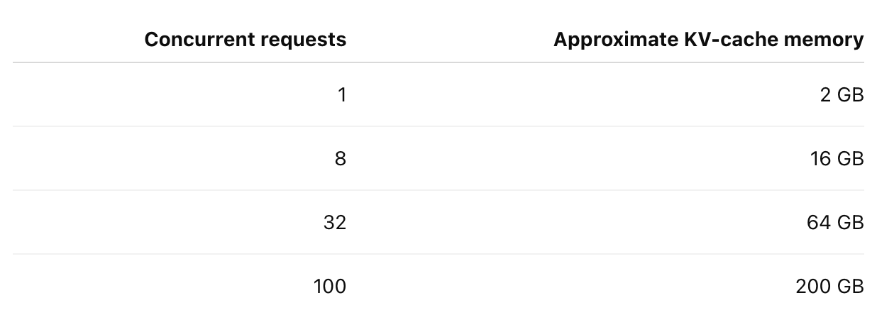
This is a simplified example, and newer architectures often use techniques such as grouped-query attention to reduce the number of KV heads. Different models can therefore have very different KV-cache requirements.

But the multiplication problem doesn’t go away.

Longer context uses more memory. More concurrent users use more memory. If both increase at the same time, the requirement can get disgusting remarkably quickly.

This is the key economic distinction.

The provider can load one copy of the model weights and use those weights to serve an entire batch of users. The same matrices participate in every request.

The KV cache contains the context of an individual request. Your giant coding repository, tool outputs and chain of agent messages aren’t the same as the context belonging to the user next to you.

Each active sequence therefore needs its own growing cache.

Suppose an 80 GB GPU uses 70 GB for the model weights. The model fits, but only 10 GB remains for the KV cache, temporary activations, communication buffers and the inference engine itself.

At that point, the provider may technically be able to load the model while still being unable to serve many people. A few users with long contexts can consume the remaining memory surprisingly quickly.

This is why serving frameworks care so much about KV-cache capacity. vLLM calculates how many tokens and concurrent requests can fit based on the memory allocated to the cache. If that space is too small, concurrency falls even though the model weights themselves fit perfectly.

Once the available KV-cache memory is exhausted, the inference engine has a few choices:

• Queue new requests until existing ones finish.

• Reduce the number of requests processed together.

• Limit the maximum context length.

• Evict cache blocks and recompute them later.

• Move some blocks into system RAM or storage.

• Spread the cache across additional GPUs.

Once again, every option comes with a cost.

vLLM supports KV-cache offloading into slower memory tiers. Completed cache blocks can live in CPU memory and return to the GPU when they’re needed again. This can be useful for multiturn conversations that pause between messages.

But an actively generating request keeps reading its KV cache during every decode step. If the required blocks live somewhere slower, the GPU may have to wait for them just like it waits for offloaded model weights.

Providers can also store the cache at lower precision. NVIDIA has shown how quantizing KV caches can reduce both their memory footprint and the bandwidth needed to read them. That allows longer contexts or more simultaneous users, although lower precision can introduce its own accuracy and implementation tradeoffs.

Prefix caching provides another useful optimization. If several requests begin with the exact same system prompt, codebase or document, the server can reuse the KV blocks it already calculated for that shared prefix. vLLM documents this as automatic prefix caching.

But most conversations eventually diverge. Once two agents start taking different actions and receiving different tool results, their new KV-cache blocks become unique.

The provider is right back to storing a separate trail of temporary state for each one.

I’ll probably write a longer post on KV-caches at some point. There a number of things you can do at both the model and application layer to overcome the constraints around them.

This gives us a better way to think about inference memory:

The weights are mostly fixed. Load the model and they occupy roughly the same amount of memory whether one person or one hundred people use it.

The KV-cache requirement is dynamic. It grows with context length, output length and concurrency. Agentic coding makes this especially painful because agents read huge files, call tools, append the results and keep the session alive across long sequences of actions.

That’s why saying “the model fits on four GPUs” doesn’t tell us much about whether the system is actually useful.

The real questions are:

• How much memory remains after loading the weights?

• How large can each user’s context become?

• How many users can generate tokens concurrently?

• What happens when their KV caches fill the remaining HBM?

• How often does the system have to move cache blocks into slower memory?

The model weights determine whether you can load the model.

The KV cache helps determine whether anyone can actually use it at scale.

Everything we’ve covered so far explains why HBM exists.

Model weights need to stay close to the processor. Inference keeps reading those weights. The KV cache grows as users send longer prompts, and splitting a model across slower memory tiers introduces even more waiting.

If you’re designing hardware for AI, the obvious response is to put an enormous amount of extremely fast memory right next to an extremely fast processor.

That’s HBM.

It’s an incredible solution to the memory problem. It’s also the reason “I need another 80 GB of memory” can somehow turn into “I guess I’m buying another server-class GPU.”

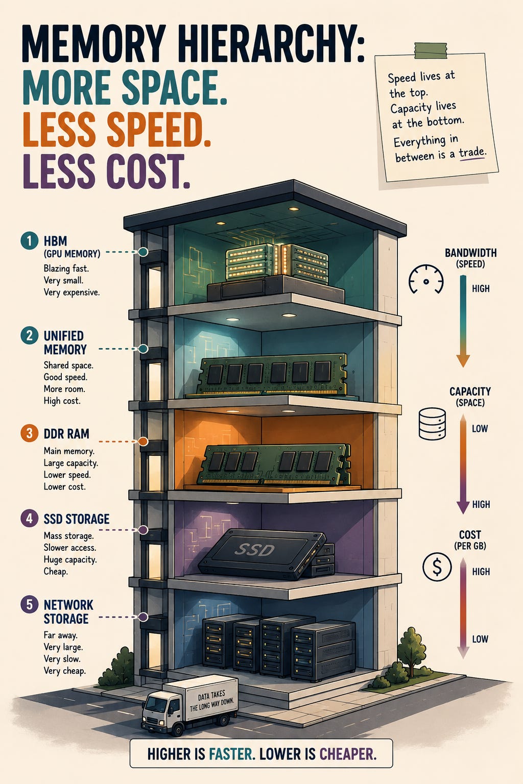
HBM stands for High Bandwidth Memory.

Like ordinary system RAM, HBM stores the data a processor is actively using. The difference is how it’s physically built and connected.

Traditional memory modules place chips beside one another on a board and communicate with the processor through a relatively narrow memory interface. HBM stacks multiple DRAM dies vertically, connects them with tiny pathways running through the silicon and packages those stacks extremely close to the accelerator.

SK hynix’s explanation of HBM describes a design with 1,024 data paths. Instead of trying to make a narrow connection run impossibly fast, HBM moves data across an extremely wide interface.

The easiest way to picture the difference is with roads.

Ordinary memory gives the processor a respectable highway. HBM builds a horrifyingly expensive mega-highway with hundreds of lanes running directly into the GPU.

That enormous connection produces enormous bandwidth. Bandwidth tells us how much data the memory can deliver each second, which is exactly what matters when a GPU is trying to read billions of model parameters over and over again.

The progression across recent NVIDIA accelerators makes the point:

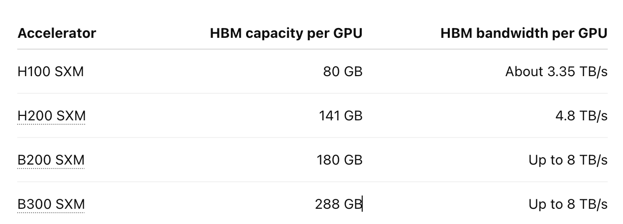
A single B200 can theoretically move the equivalent of its entire 180 GB memory capacity dozens of times per second. Real inference performance is more complicated than dividing one number by another, but that scale of bandwidth is why these accelerators can keep enormous models moving.

HBM doesn’t just hold the model. It feeds the model to the processor quickly enough for the processor’s massive amount of compute to stay useful.

GPUs are built to perform huge numbers of calculations in parallel. That makes them fantastic at the matrix multiplication inside neural networks.

But every calculation needs inputs. The GPU can’t multiply weights that haven’t arrived yet.

During low-batch decoding, the GPU may need to read a large portion of the model’s active weights to generate one token. If those weights are stored in 100 GB, 200 GB or 500 GB of memory, the speed at which memory can deliver them places a rough ceiling on token generation.

That’s why our earlier mental model was:

This isn’t a perfect performance formula. Batching, caching, quantization, kernels, attention and model architecture all affect real output speed. But it explains the basic relationship.

If a model needs to read 100 GB of active weights for each token and the memory delivers 1 TB per second, the absolute fantasy ceiling is around 10 tokens per second before accounting for anything else.

Increase the bandwidth to 4 TB per second and the processor has much more room to work. Shrink the active weights through quantization or MoE, and the same memory system can potentially generate more tokens.

The KV cache adds another stream of data. During decoding, every attention layer reads keys and values belonging to earlier tokens, uses them to calculate attention and appends new entries for the latest token. Longer contexts mean more cached data to read, and more concurrent users mean more separate caches competing for memory capacity and bandwidth.

HBM is excellent at feeding all of this data to the GPU:

• Model weights

• KV-cache blocks

• Intermediate activations

• Temporary calculation buffers

• Communication workspaces

This is why HBM isn’t just a nice feature attached to an AI accelerator. It’s part of what makes the accelerator useful.

A GPU without enough memory bandwidth is like giving someone a Formula One car and asking them to drive through Manhattan at rush hour. The engine is technically very impressive. Nobody’s going anywhere.

It’s worth pausing here because I don’t want this article to become “HBM bad.”

HBM is extremely good.

It offers several advantages at the same time:

• Enormous memory bandwidth

• High bandwidth per watt

• Short physical distances between memory and compute

• A wide interface that can feed thousands of GPU cores

• Strong performance for training and heavily batched inference

• Predictable access compared with moving weights through PCIe or storage

Building it is also genuinely difficult. Memory manufacturers stack several thin DRAM dies, align them precisely and connect them using thousands of vertical electrical paths called through-silicon vias, or TSVs.

SK hynix explains that TSVs pass vertically through tiny holes in the memory dies, connecting the stack from top to bottom. That stack then has to be packaged with the accelerator through an advanced integration process.

This is very different from buying another RAM stick and clicking it into a slot.

The GPU, the HBM stacks, the interposer, the package and the cooling system all have to work together as one tightly integrated product. Increasing HBM capacity affects package size, heat, signal integrity, power and manufacturing yield.

That complexity is part of why HBM is so fast.

It’s also part of why HBM is expensive, capacity constrained and difficult to scale casually.

The first part of the HBM tax is simple: you generally can’t buy HBM by itself and add it to your server later.

HBM is packaged with the accelerator. If you buy an H100 with 80 GB, that GPU has 80 GB. You can’t open the server six months later and slot in another 64 GB because your users started pasting larger repositories into their coding agents.

Your options are usually to:

• Quantize the model more aggressively.

• Reduce context length or concurrency.

• Offload data into slower memory.

• Add another accelerator.

• Replace the accelerator with one that has more HBM.

That last option is why the memory tax becomes a hardware tax. If you need more fast memory, you often have to buy more compute along with it.

Imagine your deployment needs another 80 GB of HBM capacity but has already got enough arithmetic performance. You can’t purchase a standalone 80 GB HBM expansion module. You purchase another GPU, another share of a GPU server or additional cloud instances.

You’re not only buying memory. You’re also paying for:

• More tensor cores

• More power delivery

• More cooling

• More rack space

• More networking

• More orchestration

• More things that can randomly ruin someone’s weekend

This is a strange way to buy memory.

It would be like discovering that your laptop needs another terabyte of storage and being told that the only available upgrade is a second laptop.

The second part of the tax is unused capacity. A workload may need the GPU’s memory bandwidth without fully using all its compute, or it may need the memory capacity while tolerating much lower bandwidth.

In either case, the memory and compute arrive as a bundle. You pay for the whole package even when your workload mainly cares about one part of it.

Let’s take a hypothetical model whose quantized weights occupy 500 GB.

Ignoring the KV cache and every other runtime expense, the absolute arithmetic minimum would be:

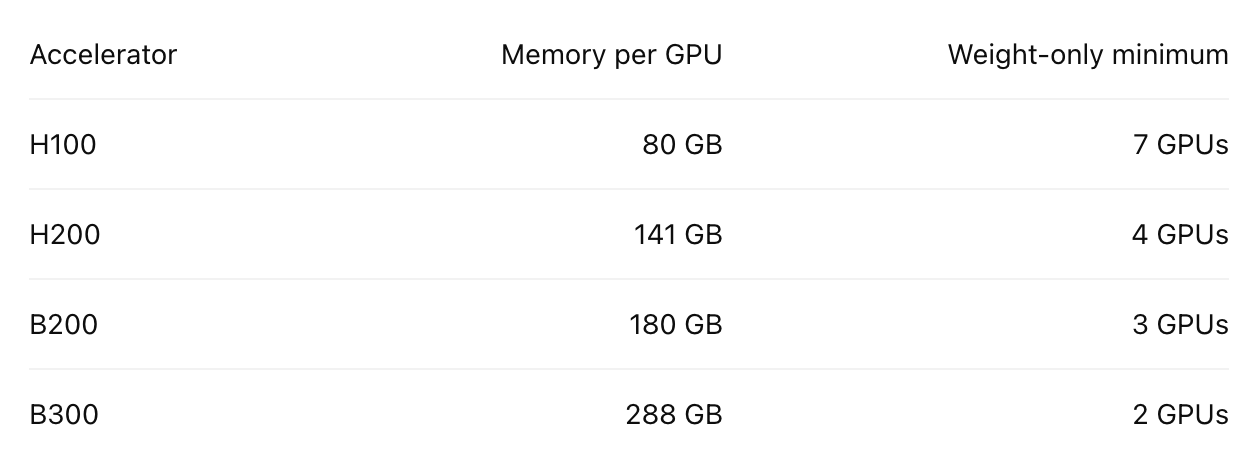
That looks almost manageable until we remember everything from Part 3.

The model weights aren’t the only resident in memory. We still need room for:

• The KV caches belonging to active users

• Temporary activations and buffers

• Quantization metadata

• Communication workspaces

• The inference runtime

• Memory fragmentation

• Enough headroom to prevent the server from falling over

Seven H100s provide 560 GB of total HBM, leaving only 60 GB after loading 500 GB of weights. Spread across seven devices, that remaining memory has to support every cache, buffer and user request.

Technically fitting is not the same thing as having a production-ready deployment.

In practice, you might move to eight GPUs because that’s a common server configuration and it gives the system more breathing room. Now your 500 GB model is running on an entire eight-GPU HGX system before we’ve even discussed redundancy or replicas.

If you need a second copy for additional throughput, that’s another eight GPUs. If you need failover capacity, add more. If you need separate fleets for several model versions, keep going until the data center sales rep starts sending you a Christmas card.

The GPUs also have to communicate. Tensor parallelism needs frequent synchronization. Expert parallelism routes tokens between devices. Pipeline parallelism passes activations from one stage to another.

So adding GPUs creates more than a hardware bill. It creates a networking and coordination bill too.

This is why the number of parameters can have such an outsized effect on inference economics. A model that’s 20% larger may cross a hardware boundary and force the provider to add an entire accelerator, change its partitioning strategy or move to a larger server.

Capacity comes in chunks.

If a model needs 81 GB and your GPU has 80 GB, you don’t have a 1 GB problem. You’ve potentially got a second-GPU problem.

AI infrastructure is usually described as a compute race. Companies talk about FLOPS, tensor cores, training clusters and how many GPUs they plan to install.

But inference doesn’t only consume compute. It consumes a combination of:

• Arithmetic

• Memory capacity

• Memory bandwidth

• Communication bandwidth

• Power

A provider may rent an H100 because it needs the compute. It may rent one because it needs 80 GB of fast memory. It may rent eight because the model needs 500 GB and has to live somewhere.

Those are very different reasons to buy the same hardware.

This is the hidden tax at the center of model inference. The most valuable feature of an expensive accelerator may not be how quickly it performs math. It may be that hundreds of gigabytes of extremely fast memory are packaged beside that math.

HBM solves a difficult engineering problem brilliantly. It keeps enormous processors fed, prevents constant trips into system RAM and makes large-model inference fast enough to feel interactive.

But brilliance and economic efficiency aren’t always the same thing.

Sometimes you’re buying the GPU for its math. Sometimes you’re buying an extremely expensive memory card that happens to contain a GPU.

And once you need several of those memory cards to hold one model, the connections between them become part of the machine.

That’s where things get even more fun.

At the end of Part 4, we took a 500 GB model and spread it across several GPUs. The model finally fit, but we quietly created another problem.

Those GPUs now have to behave like one machine.

Each GPU owns a different piece of the model and keeps it inside the memory physically attached to it. As a token moves through the distributed model, the devices exchange activations, partial calculations, routed tokens and sometimes KV-cache data.

The connections carrying that traffic are called interconnects. Once the model spans several pieces of hardware, those connections stop being background plumbing. They become part of the inference engine.

The model’s full weights don’t normally bounce between devices for every token. That would be unbelievably slow and defeat the point of splitting it.

Instead, each device keeps its assigned weights resident in its own memory. The system only moves the intermediate data needed to connect one piece of the calculation to the next.

What moves depends on how the model was divided:

• Pipeline parallelism moves activations. One device finishes its group of layers and sends the resulting activations to the next stage. Communication happens less frequently, but every stage depends on the one before it.

• Tensor parallelism moves partial results. Several devices work on the same layer and combine their answers before continuing. This requires frequent operations such as all-reduce, all-gather and reduce-scatter.

• Expert parallelism moves routed tokens. Tokens travel to whichever devices hold their selected experts. The results then travel back and get combined.

• Disaggregated serving can move KV-cache blocks. One group of devices processes the prompt, while another generates the response. The request’s temporary attention state has to travel between them.

Tensor parallelism is usually the most communication-sensitive of these approaches. A tiny delay becomes painful when the model pays it across dozens of layers and every generated token.

Expert parallelism creates a different problem. If one expert becomes unusually popular, the device holding it can receive far more tokens than the others. The network may have plenty of total bandwidth while one connection still becomes a traffic jam.

Moving the KV cache can be especially expensive for long-context and agentic workloads. NVIDIA’s documentation on distributed inference transfers calls it out as a critical part of modern inference infrastructure.

The conversation looks like one continuous session to the user. Underneath, its temporary memory may be taking a road trip between servers.

Here’s the physical detail that makes all of this important: HBM belongs to the accelerator it’s attached to.

An H100’s 80 GB of HBM sits beside that H100. An H200’s 141 GB sits beside that H200. A B200’s 180 GB sits beside that B200.

Each GPU can read from its own attached HBM at enormous speed. But when a model is split across several GPUs, those memory pools don’t magically melt together into one enormous bucket.

Four B200s may contain 720 GB of HBM in total, but they still contain four separate 180 GB pools.

If GPU 1 needs information stored beside GPU 4, it has to request that information across an interconnect. The memory may still be HBM, but it’s remote from the GPU doing the calculation.

Think of each GPU as its own state. Inside every state, HBM is a massive fucking freeway with thousands of lanes. Data flies between the local memory and the local processor at several terabytes per second.

Now imagine connecting those states with a much smaller bridge. The internal freeways are still enormous, but anything crossing a state line has to squeeze through the bridge.

That’s why adding another GPU isn’t the same as extending the memory of the first one. You’re adding another island of fast memory and building a bridge to it.

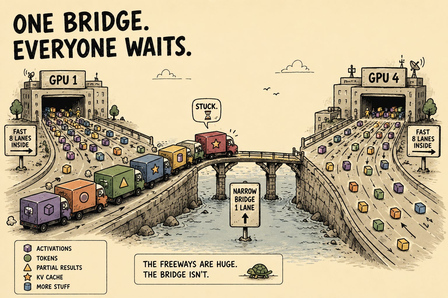
Inside a B200, its attached HBM can deliver up to 8 TB per second to that GPU’s compute cores.

If the same GPU needs data held beside another GPU, the transfer has to cross an interconnect. Blackwell NVLink provides up to 1.8 TB per second of bidirectional bandwidth per GPU.

That’s remarkably fast. It’s also far less bandwidth than the GPU has inside its own hardware.

The bridge narrows again when data travels between servers. A 400G ConnectX-7 adapter provides 400 gigabits per second, which converts to 50 gigabytes per second before overhead.

Thunderbolt 5 sits below those data-center interconnects, but one “10 GB/s” figure doesn’t tell the whole story. A single connection provides 10 gigabytes per second in each direction simultaneously, or 20 gigabytes per second of aggregate bidirectional bandwidth.

Apple’s distributed stack can also use two or three parallel Thunderbolt links between neighboring Macs. That multiplies the theoretical bandwidth available between those machines before overhead.

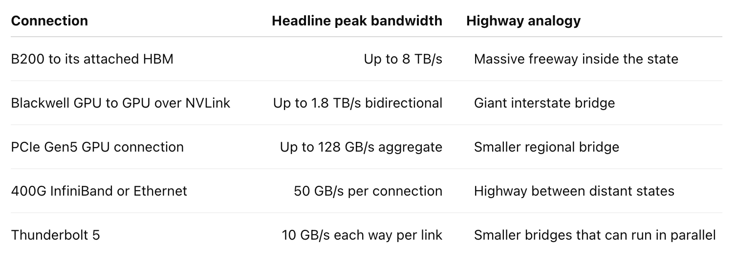
These are headline specifications, not guaranteed application throughput. Vendors don’t always report bandwidth in the same way, and real systems lose performance to protocols, coordination and imperfect traffic patterns.

The exact numbers matter less than the hierarchy. The farther data travels from the processor that needs it, the narrower the road generally becomes.

Distributed inference works by minimizing how much data crosses those bridges. The software tries to move activations instead of weights, avoid unnecessary transfers and overlap communication with useful computation.

HBM gives every accelerator an extraordinary internal freeway. The interconnect determines how badly traffic backs up at the state line.

PCIe is the general-purpose connection inside most servers. GPUs, network cards and storage devices use it to communicate with the CPU and the rest of the machine.

It’s fast by ordinary computer standards. AI infrastructure is not an ordinary workload.

Tensor parallelism can require devices to exchange partial results inside many model layers. If every exchange travels through PCIe, communication may consume much of the time saved by spreading the calculation across more GPUs.

NVIDIA created NVLink and NVSwitch to give GPUs a much faster and more direct path. NVLink provides high-bandwidth GPU-to-GPU communication, while NVSwitch connects multiple GPUs into a larger fabric.

A Hopper GPU can provide up to 900 GB per second of NVLink bandwidth. Blackwell raises that to 1.8 TB per second bidirectionally.

This doesn’t merge every HBM stack into one physically shared pool. It builds much larger bridges between the separate pools, letting the GPUs behave more like one tightly connected system.

That’s also why the GB200 NVL72 isn’t simply a rack containing 72 independent GPUs. It’s 72 GPUs, dozens of separate HBM pools and a massive NVLink fabric designed to hold the whole thing together.

NVIDIA describes it as acting like one massive GPU. The word “like” is doing some work there.

Bandwidth tells us how much data a connection can move over time. Latency tells us how long it takes for one transfer or coordinated operation to begin and complete.

A delivery truck can carry an enormous amount of furniture, giving it excellent bandwidth. If the truck takes three hours to arrive, it still has terrible latency.

Large transfers care about bandwidth. Small, frequent synchronization operations often care more about latency because the devices repeatedly stop and wait for one another.

During decoding, those waits sit directly in the user’s path. The model can’t finish token 101 before token 100 exists.

If each token requires several rounds of cross-device synchronization, tiny delays get multiplied across many layers and thousands of generated tokens.

Real communication performance depends on:

• The size of each transfer

• How often communication occurs

• Whether transfers overlap with computation

• How many devices participate

• Which collective operation is being used

• How quickly every device reaches the synchronization point

The specification tells you how wide the road is. It doesn’t tell you how many toll booths someone put on it.

Total bandwidth also hides the shape of the network.

Imagine four devices connected in a line:

Device 1 ↔ Device 2 ↔ Device 3 ↔ Device 4

Device 1 can talk directly to Device 2. If it needs data from Device 4, that data may have to travel through the middle of the system.

A mesh gives devices more direct connections. A ring uses fewer links but sends nonadjacent traffic through intermediate nodes. A tree moves data through layers of switches, while a fully connected fabric gives every device a fast path to every other device.

Different workloads prefer different shapes:

• Tensor parallelism benefits from direct, low-latency paths because communication happens repeatedly inside the model.

• Pipeline parallelism can tolerate simpler connections because activations only move between stage boundaries.

• Expert parallelism benefits from strong all-to-all connectivity because routed tokens may need to reach any device.

• Large collective transfers may benefit from a ring that combines several links between neighboring devices.

This is why “we have sixteen GPUs” doesn’t tell you nearly enough. Sixteen GPUs connected through the right topology can form a powerful inference system.

Sixteen GPUs connected badly can form an expensive group chat where nobody knows whose turn it is to speak.

Distributed inference requires devices to coordinate. If eight GPUs work on pieces of the same layer, the model usually can’t continue until every required piece is ready.

Seven GPUs can finish on time, but if the eighth is delayed, the others may have to wait. That delayed device is called a straggler.

A device can become a straggler because it received more MoE tokens, encountered a slower memory transfer or competed with another process for bandwidth. It could also have a congested network path or simply own a heavier model shard.

At small scale, these differences may barely matter. Across many devices and repeated synchronization points, they accumulate.

The probability that at least one device is having a weird moment grows with the cluster. This is the distributed-systems version of planning dinner for twenty people. Someone will be late, someone will be lost and someone apparently didn’t see the group text.

Good inference software reduces the damage through balanced partitioning, smarter routing and overlapping communication with computation. It can’t remove coordination from a workload that depends on several devices producing one answer together.

Thunderbolt 5 is slower than the specialized fabrics connecting data-center GPUs. The interesting part is how efficiently modern Macs can now use it.

Starting with macOS 26.2, Apple added RDMA over Thunderbolt. RDMA stands for Remote Direct Memory Access, and it lets one machine move data directly into another machine’s memory while avoiding most CPU and operating-system overhead.

Without RDMA, a transfer may involve several copies and layers of software coordination. Data gets placed into a network buffer, processed by the operating system, moved across the link and copied into another buffer on the receiving machine.

That’s a lot of ceremony around moving bytes.

Returning to our freeway analogy, ordinary networking is like forcing every car to exit the highway, stop at customs, unload its cargo, reload it into another car and then continue into the next state.

Thunderbolt RDMA doesn’t make the bridge infinitely wide. It creates an express lane that lets the cargo cross without stopping at customs.

This becomes especially interesting on Apple Silicon because each Mac has a large pool of unified memory shared by its CPU and GPU. Several high-memory Macs can keep model shards resident in their own memory while using Thunderbolt RDMA to exchange activations and partial results.

Apple demonstrates this workflow in its distributed MLX session. Four M3 Ultra systems are connected through Thunderbolt 5, RDMA is enabled and MLX shards models across the cluster.

The stack has three important pieces:

• Thunderbolt 5 provides the physical links.

• RDMA moves data directly between the memory of different Macs.

• JACCL and MLX handle collective communication and model sharding.

Apple’s JACCL library also understands that no topology is perfect. A full mesh gives every Mac a direct path to every other Mac, reducing latency for small and frequent messages.

A ring connects each Mac only to its neighbors. Nonadjacent communication takes additional hops, but the unused ports can run two or three parallel Thunderbolt cables between each neighbor.

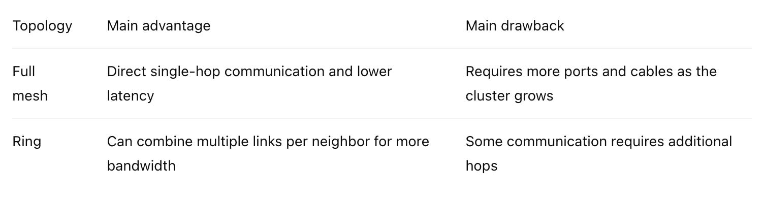
JACCL can choose between mesh-like and ring communication patterns based on the message size and collective operation. Small messages tend to care more about latency, while larger transfers benefit from several links operating in parallel.

This isn’t merely theoretical. In Apple’s four-Mac example, MLX sharded a 27-billion-parameter model across four M3 Ultras and generated tokens at nearly three times the rate of one machine.

Apple also demonstrated a trillion-parameter model that couldn’t fit on one M3 Ultra running across four of them. The exact speedup depends on the model, quantization, topology and parallelism strategy, but the result shows that a consumer interconnect doesn’t need to match NVLink before it becomes useful.

Thunderbolt RDMA still doesn’t turn four Macs into one chip or create one physically shared memory pool. Tensor parallelism can also saturate those links because it communicates inside many layers.

What it does is let relatively accessible machines communicate far more efficiently than ordinary consumer networking would suggest.

The bridge is still smaller than the freeway. But it’s direct, several bridges can run in parallel and the cars no longer have to stop at customs.

That’s pretty damn useful.

Suppose someone tells you their cluster has one terabyte of memory. That could mean one processor has direct access to a terabyte of unified memory, eight GPUs each have a smaller pool of HBM connected through NVLink or several consumer machines communicate through Thunderbolt RDMA.

All three systems may contain the same number of bytes. They won’t perform the same way.

To understand whether distributed memory is useful, we need to ask:

• Which processor owns each piece of memory?

• How quickly can another processor access it?

• How many links connect the devices?

• How many hops does each transfer require?

• Is the system moving weights, activations or KV-cache blocks?

• How frequently do the devices synchronize?

• Can communication overlap with computation?

Memory capacity tells us whether all the pieces of the model can fit somewhere in the system. The interconnect tells us whether those pieces can cooperate quickly enough to feel like one model.

HBM gives each GPU extraordinary access to its own attached memory. NVLink and InfiniBand combine those GPUs into incredibly fast but incredibly expensive systems.

Thunderbolt RDMA creates a cheaper bridge between machines with large unified-memory pools. It comes with less bandwidth, so it requires smarter choices about partitioning, communication and topology.

Can slower and cheaper memory ever produce better inference economics?

That’s where we’re going next.

After everything we’ve covered, this sounds like a ridiculous question.

HBM is dramatically faster than ordinary RAM. It sits beside the accelerator, feeds the processor at several terabytes per second and powers the fastest AI systems in the world.

Why would we ever replace it with slower memory?

Because “fastest” and “best economics” aren’t always the same thing.

The wrong question is whether DDR, LPDDR or unified memory can beat HBM in a raw bandwidth contest.

They can’t.

The right question is:

Does every inference workload need HBM-level bandwidth badly enough to justify HBM-level cost?

Some workloads absolutely do. Training giant models, serving enormous batches and chasing maximum single-request speed are perfect jobs for HBM.

Other workloads may care more about fitting a capable model into one large memory pool, supporting a predictable number of users and producing useful answers at a reasonable speed.

In those cases, a system that’s slower per token but dramatically cheaper to own can become very interesting.

HBM is optimized for bandwidth. DDR, LPDDR and unified-memory systems can offer much more capacity per machine at a lower cost, but they deliver that data more slowly.

That tradeoff becomes obvious when we compare recent hardware:

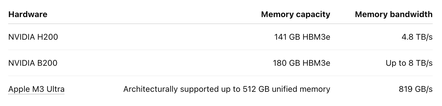
The B200 has nearly ten times the memory bandwidth of the M3 Ultra. If the goal is to push one model through an enormous batch as quickly as possible, that difference is absolutely brutal.

But the M3 Ultra architecture can address far more memory from one processor. Apple originally offered up to 512 GB of unified memory in a single Mac Studio.

That creates a different advantage. A model that requires several HBM-equipped GPUs may fit inside one unified-memory machine without being divided at all.

You’ve traded bandwidth for capacity, but you may also have avoided tensor parallelism, cross-GPU synchronization and an entire pile of expensive networking.

Imagine a quantized model whose weights occupy 150 GB.

That model doesn’t fit inside an 80 GB H100. It doesn’t fit inside a 141 GB H200 either, especially once we leave room for the KV cache and runtime overhead.

The obvious HBM solution is to split the model across several GPUs. That gives us enormous local bandwidth, but it also introduces the communication tax from Part 5.

A system with several hundred gigabytes of unified memory can keep the entire 150 GB model inside one memory pool. It won’t read those weights as quickly as a B200, but it also won’t synchronize several GPUs while generating every token.

That doesn’t automatically make the unified-memory machine faster. It usually won’t be.

It can make the system much simpler and potentially much cheaper:

• One copy of the model stays resident.

• No tensor results have to cross GPU boundaries.

• No NVLink or InfiniBand fabric is required.

• The KV cache can use the same large memory pool.

• The provider isn’t buying several accelerators just to combine their memory.

The fastest individual components don’t always create the best overall system. Sometimes eliminating an expensive boundary matters more than making everything on either side of it absurdly fast.

Mixture-of-experts models separate two ideas that dense models keep tied together.

The total parameter count largely determines how much memory the complete model needs. The active parameter count helps determine how many weights participate in processing each token.

A model might contain hundreds of billions of parameters while activating only a small fraction of them for each token. All the experts still need to live somewhere, but the processor doesn’t read every expert during every pass.

That creates an unusual workload:

• It needs lots of memory capacity to hold the full expert library.

• It needs enough bandwidth to read the selected experts quickly.

• It may not need to stream every byte of the complete model for every token.

This is exactly where a large pool of slower memory can become compelling. The hardware can keep the entire model resident while the router activates a much smaller working set.

It’s not free. Expert selections can be irregular, popular experts can create hotspots and the shared dense layers still participate in every token. The relationship between active parameters and bytes read is also more complicated than one clean number.

But the basic economics change. MoE lets a model demand enormous capacity without necessarily demanding bandwidth proportional to its total size on every token.

HBM is designed to solve both problems at the maximum possible speed. A cheaper architecture can ask whether the workload really needs that much speed for every stored parameter.

Infrastructure discussions tend to treat the fastest system as the winner. Users don’t always think that way.

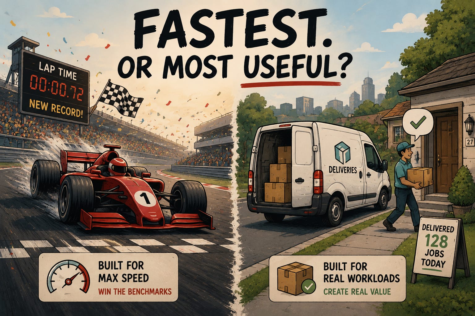
A coding agent producing 70 tokens per second is obviously better than one producing 10. But the difference between 10 and 20 tokens per second may matter far more than the difference between 70 and 100.

At some point, the model becomes fast enough for the workflow.

This threshold depends on the use case:

• Interactive chat feels sensitive to pauses and slow token delivery.

• Coding agents spend time calling tools, reading files and running tests.

• Background research tasks may run for several minutes without anyone watching.

• Batch document processing may care about total daily throughput rather than one response.

• Internal enterprise workflows may prioritize privacy and predictable cost.

An agent that waits fifteen seconds for a test suite doesn’t need the model generating at 200 tokens per second during that wait. A background task doesn’t care whether its explanation appeared beautifully one token at a time.

The useful question isn’t always “How fast can this hardware generate?” It may be “Is it fast enough that model generation is no longer the biggest delay in the workflow?”

Once the answer is yes, paying much more for additional speed can produce rapidly diminishing value.

Single-stream token generation is easy to understand, so it dominates hardware comparisons. Serve one request, measure its speed and declare a winner.

Real providers don’t serve one perfectly behaved request forever.

Users arrive at different times, send prompts of different lengths and pause while their agents call tools. Some requests are processing giant contexts, while others are decoding short answers.

A good scheduler can use those gaps. It can batch compatible requests, keep processors busy and route work toward machines that have available memory.

Batching is especially important because multiple requests can reuse the same loaded weights. The system reads a block of model weights and applies it across several sequences before moving onward.

This increases the amount of useful calculation performed for each byte fetched from memory. A workload that looked completely bandwidth-bound at batch size one may use the hardware far more efficiently at a larger batch.

Cheaper memory doesn’t magically gain more bandwidth. But better batching, request routing and concurrency management can extract more useful work from the bandwidth it has.

That shifts the question from:

How quickly can one user consume the entire machine?

To:

How much useful work can the machine complete across all its users?

Those are very different benchmarks.

Large pools of DDR, LPDDR or unified memory become most interesting when the workload has several of these characteristics:

• The model is heavily quantized.

• The model uses MoE and activates a relatively small working set.

• The complete model can stay resident without SSD offloading.

• Moderate per-user decode speed is acceptable.

• Several requests can be batched or scheduled efficiently.

• Aggregate throughput matters more than one record-setting stream.

• Privacy or local ownership matters.

• Hardware cost matters more than benchmark leadership.

A system like this isn’t trying to beat an NVL72 at its own game. That would be deeply silly.

It’s trying to serve a useful model at acceptable speed without paying for an entire rack of HBM and the fabric required to hold it together.

That’s a different game.

There are also workloads where cheaper memory is simply the wrong answer.

HBM remains extremely difficult to beat when:

• Maximum single-request speed is essential.

• Training or heavy fine-tuning is the primary workload.

• Large batches need maximum aggregate throughput.

• The model uses dense computation across most of its parameters.

• Tensor parallelism requires frequent collective operations.

• Long contexts create enormous, constantly accessed KV caches.

• The processor can consume data much faster than cheaper memory supplies it.

Training is the clearest example. During training, the system stores weights, gradients, optimizer state and activations while performing huge amounts of parallel computation.

That workload can use every bit of bandwidth and compute modern accelerators provide. Replacing HBM with slower memory would leave expensive compute cores waiting.

High-volume inference can create a similar result. Once a provider has enough concurrent demand to keep giant batches full, HBM’s bandwidth can be spread across many users.

The expensive GPU starts earning its keep.

The argument isn’t that HBM is wasteful. It’s that HBM is optimized for a performance envelope that not every inference deployment occupies.

Tokens per second is useful. It tells us how quickly a model generates output under a particular configuration.

It doesn’t tell us whether the system makes economic sense.

A provider should also care about:

• Tokens per second per dollar: How much throughput does the hardware produce relative to its cost?

• Concurrent users per dollar: How many people can receive acceptable service from the system?

• Memory capacity per dollar: How much model and KV-cache state can remain resident?

• Cost per completed task: How much does it cost to finish an actual coding, research or document workflow?

• Power per generated token: How much energy does the system consume while producing useful output?

• Utilization: How much of the purchased hardware is doing valuable work?

• Quality-adjusted cost: How much does it cost to get a result from a model capable of completing the task correctly?

That last metric matters more as smaller open models approach frontier performance.

If a less expensive model solves 95% of the same coding tasks, serving it cheaply may matter more than squeezing another 10% of raw speed from the hardware.

Nobody buying AI infrastructure actually wants tokens. They want pull requests, reports, support resolutions, completed workflows and fewer engineers screaming at their usage bill.

The token is just the intermediate product.

An HBM system may generate more tokens per second, finish a benchmark faster and support a larger batch. It can win every obvious performance comparison.

A cheaper-memory system may still offer:

• More resident model capacity per dollar.

• More KV-cache headroom.

• Lower power consumption.

• Simpler deployment.

• Less reliance on scarce accelerators.

• Better economics at moderate utilization.

• Enough performance for the actual workload.

That’s the central argument.

The goal isn’t to prove that slower memory is secretly faster. It isn’t.

The goal is to find the cheapest byte of memory that’s still fast enough.

For some workloads, that byte lives in HBM. For others, it may live inside a large unified-memory system or across several consumer machines connected through a carefully designed interconnect.

The interesting part isn’t picking one universal winner. It’s matching the memory architecture to the workload instead of treating the most expensive option as the default.

And yes, this is where I’m about to shamelessly plug what we’re building.

Sorry. We’ve got bills to pay. 😅

This whole memory problem is a big part of what we’re working on at CueCloud.

We’re exploring whether large open models can be served across consumer-grade hardware with enormous pools of relatively affordable memory, without depending entirely on scarce and painfully expensive HBM.

The bet isn’t that consumer memory is secretly faster than HBM. It isn’t. HBM is an absolute monster, and if your only goal is generating tokens as quickly as physically possible, it’s probably still what you want.

Our bet is that plenty of real inference workloads don’t need the fastest memory on Earth. They need:

• Enough memory to keep the model’s weights available

• Enough bandwidth to generate tokens at a useful speed

• Enough interconnect performance to split work across multiple machines

• Software that knows where every layer, expert and KV-cache block should live

• Scheduling that keeps the hardware busy instead of chasing a flashy single-user benchmark

That last part is where this gets genuinely hard. Buying a bunch of machines with lots of memory doesn’t magically turn them into one giant computer. The software still has to partition the model, balance the workload and prevent the interconnect from becoming a tiny bridge between several massive fucking freeways.

It also has to handle all the boring production problems. Requests need to be routed. Compatible workloads need to be batched. KV-cache pressure needs to be managed. Machines will fail, users will show up at the same time and someone will inevitably try to stuff a small novel into the context window.

If you can solve those problems, though, the economics start looking very different. Instead of asking how many extremely expensive GPUs you need to fit a model, you can start asking how much affordable memory you can combine while keeping performance inside the range people actually care about.

That’s the distinction this entire article has been building toward. The best system isn’t always the one with the highest memory bandwidth or the fastest single-user token rate. Sometimes it’s the one that can fit the model, serve a useful number of people and complete real work without setting a pile of money on fire.

HBM will remain essential for training, giant batches and workloads where every millisecond matters. But inference is a much bigger and messier market than that. There’s an enormous middle ground where “fast enough” paired with dramatically better economics could win.

That’s the CueCloud bet.

We’re not trying to build the fastest memory system on Earth. We’re trying to find the cheapest byte of memory that’s still fast enough.