Training Sparse Autoencoders

A language model’s residual stream is a high-dimensional vector at every token position. Most of that space is opaque: thousands of dimensions mixing syntax, facts, style, and safety behavior into a single point. A SAE is trained to reverse that compression. It learns a dictionary of feature directions such that any activation can be written as a sparse sum of a few of them. Each nonzero coefficient is a hypothesis about what the model is representing at that moment.

Public SAE releases exist for some catalog models. Aquin also supports training on whatever is loaded in your session: GPT-2, Llama, BERT-style encoders, fine-tuned checkpoints. The training problem is the same in every case. Collect activations that match the weights you care about, fit a sparse autoencoder on those vectors, then evaluate whether the resulting features are worth using before you build circuits or steering experiments on top of them.

This article is about that fit: the geometry of the training data, the optimization objective, what changes between LLMs and embedding encoders, and how dictionary quality shows up in the metrics Aquin logs during a run.

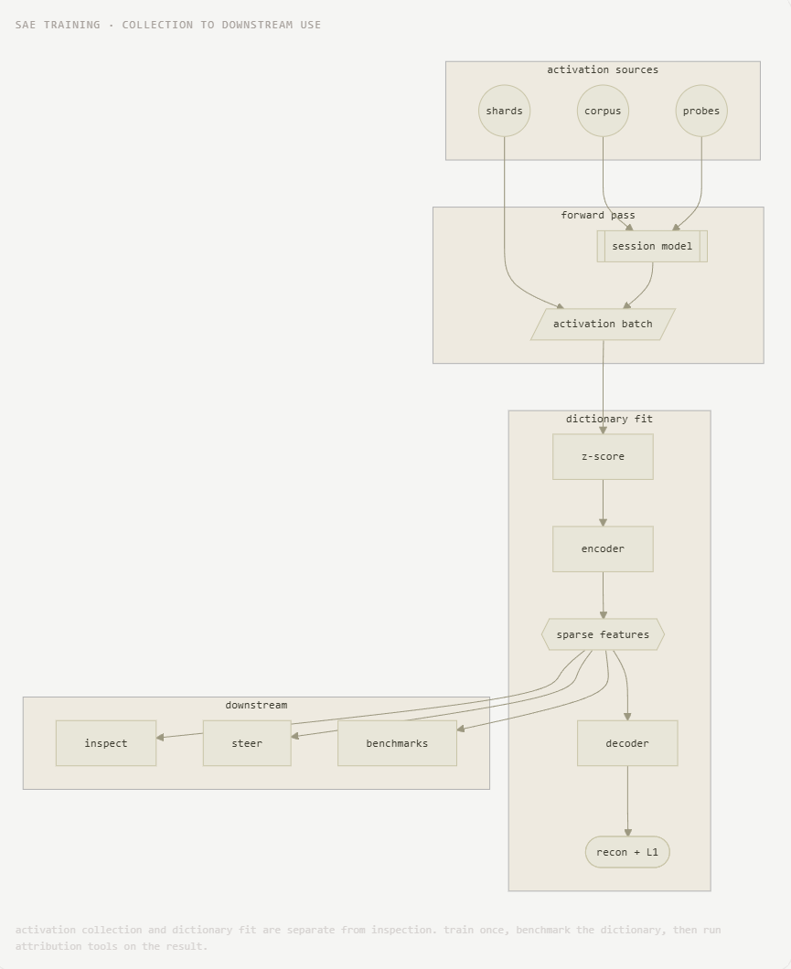
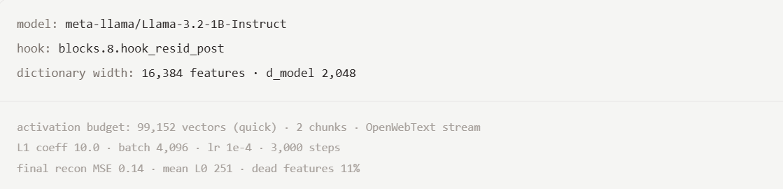
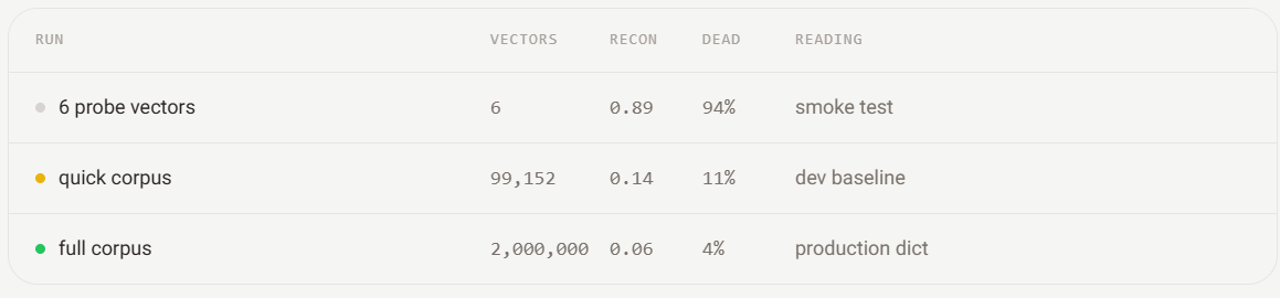
The examples below come from a quick training run on Llama 3.2 1B Instruct at layer 8: corpus collection, then 3,000 optimizer steps. The same setup was used to contrast probe-scale training (6 vectors from a generated capture) against corpus-scale collection (~99k vectors). The gap between those two runs is the central lesson of SAE training in practice.

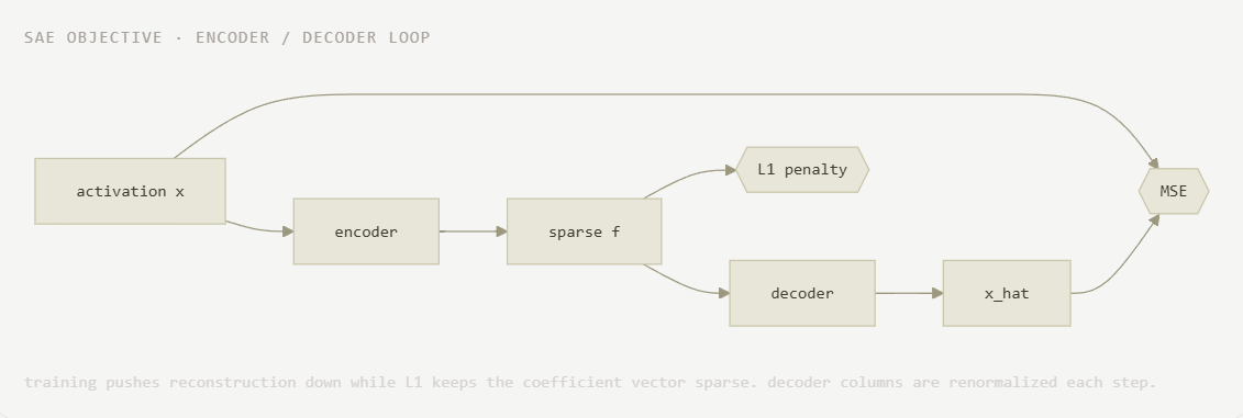
dictionary learning here means fitting an encoder and decoder on a large sample of activation vectors. The encoder maps a normalized activation to a sparse coefficient vector. The decoder maps those coefficients back to activation space. Training minimizes reconstruction loss plus an L1 penalty that pushes most coefficients to zero. Decoder columns are unit-normalized after each step so features compete on direction, not scale.

The output is not a labeled concept list. It is a set of directions in activation space. Whether a feature becomes monosemantic depends on whether the training distribution exposed the model to enough diverse contexts for that direction to specialize. Optimization can drive reconstruction down on a tiny probe set while leaving almost every feature unused. That is expected behavior, not a bug in the trainer.

Before any gradient step, Aquin materializes activations to disk as normalized chunks. Three collection modes feed the same trainer. The difference is scale and intent, not file format.

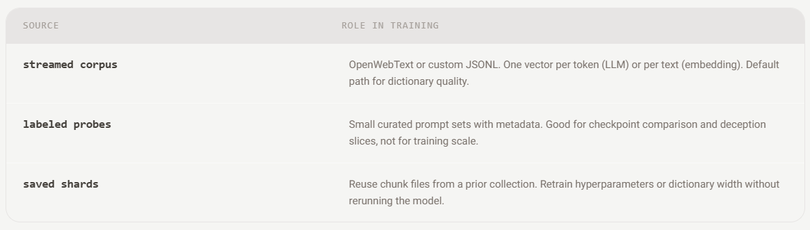
Default collection streams web text through the loaded model and records one activation vector per token position (LLM) or per input span (embedding). Quick runs target ~100k vectors. Full runs target 2M. Collection resumes if chunks already exist on disk, so interrupted runs do not repeat forward passes.

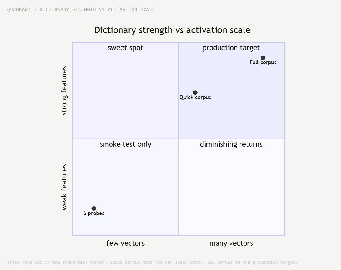
Diversity matters more than step count. A dictionary trained on six hand-picked probes can minimize loss on those six points while learning almost nothing general. A dictionary trained on 99k corpus tokens starts to separate broad syntactic and topical structure even in a quick run.

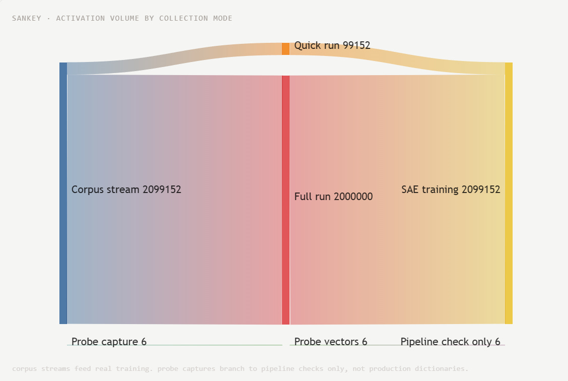
Labeled probe captures (typically 6 to 64 prompts with metadata) are valuable for comparing checkpoints, encoding deception slices, and exporting tensors with manifest provenance. They are the wrong substrate for dictionary learning. On a six-vector probe run, final reconstruction stayed high and over 90% of features never fired. The trainer converged on a trivial solution because the input distribution had no breadth.

Probe captures can still seed a training rerun when imported into chunk format, but only as a pipeline check. Production interpretation work should use corpus collection or reuse a full activation shard directory from a prior run.

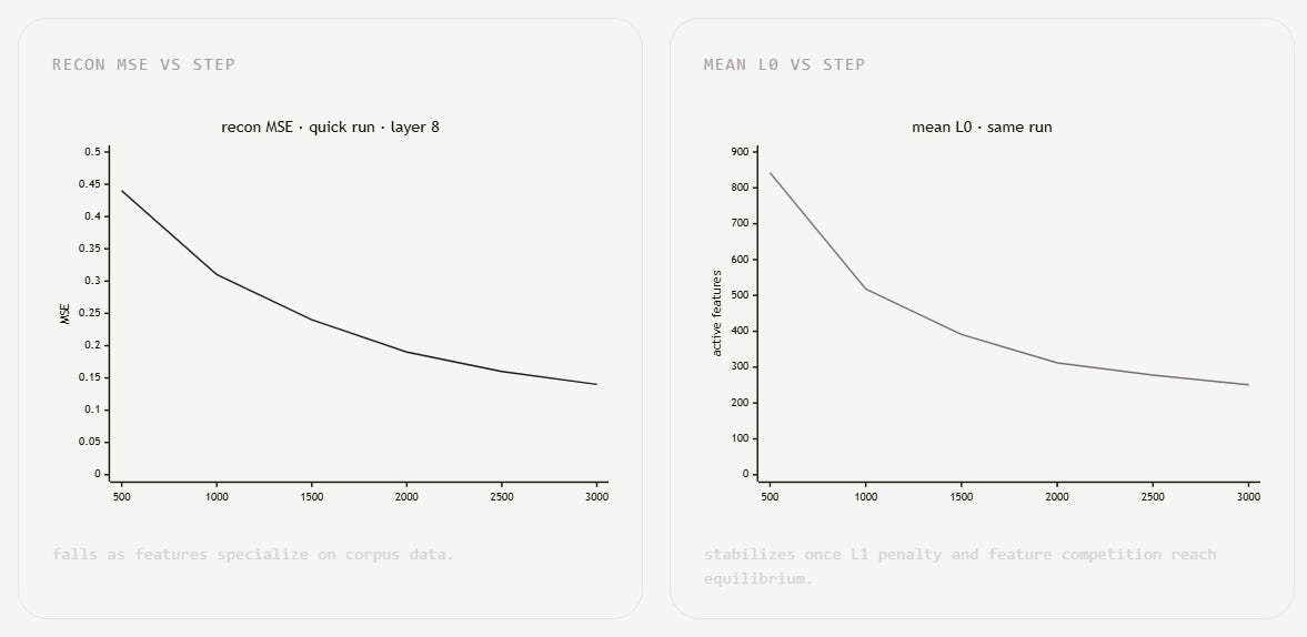
Aquin logs reconstruction MSE, mean L0 sparsity, and dead-feature count every 500 steps. On a healthy corpus run, reconstruction falls steadily while L0 settles into a band set by the L1 coefficient. Dead features drop as more directions claim territory in activation space.

The curves below are from the Llama 3.2 1B quick run at layer 8. Reconstruction above 0.4 at step 500 is normal early noise. By step 3,000 the dictionary is usable for development, though full-scale collection still improves feature semantics.

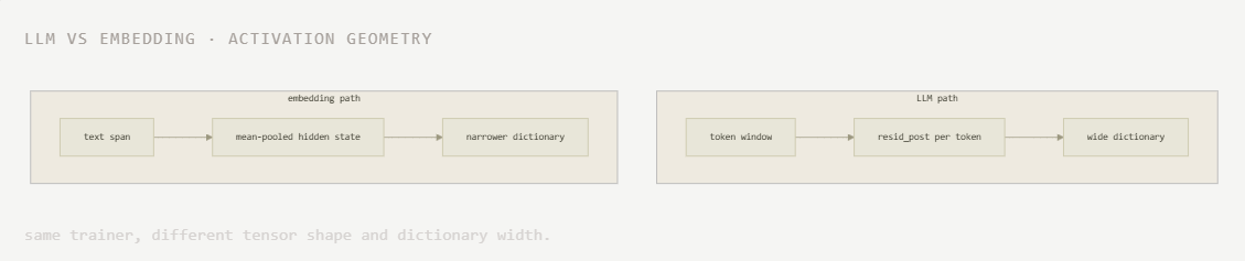
The trainer is shared. The activation tensor is not. LLMs record every token position in a fixed window from the post-block residual. Embedding encoders record one mean pooling vector per text after a forward pass through hidden states. Embedding dictionaries are narrower (4,096 features typical vs 32,768 on small LLMs) and use a lower L1 coefficient because pooled vectors are already compressed relative to per-token streams.

Feature tools differ by mode after training. LLMs get inspect, steer, and circuit graphs on token positions. Embeddings get sae-browser, contrastive decomposition, and faithfulness probes on sentence pairs. The training objective is the same; only the hook geometry and downstream readout change.

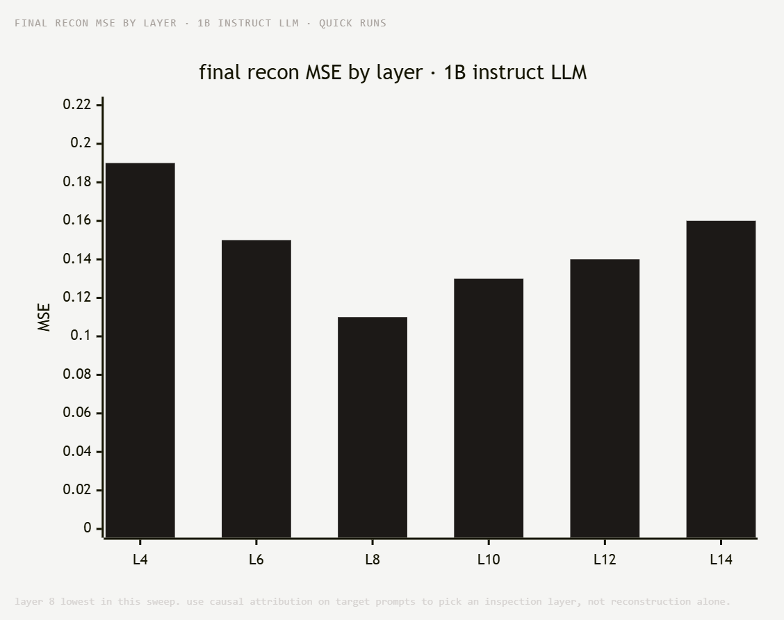
Mid-layer residuals usually give the best reconstruction-effort tradeoff on small LLMs: enough abstraction that features are semantic, not purely lexical. Early layers reconstruct easily but features tend to be syntactic fragments. Very late layers track output logits closely and can be harder to sparsify cleanly.

On quick runs across mid layers of a 1B instruct model, layer 8 reached the lowest final reconstruction in a sweep from L4 to L14. That does not mean layer 8 is always the right interpretability target. Causal tracing on your actual prompts may peak elsewhere. Train where you plan to inspect, not where reconstruction is globally minimal.

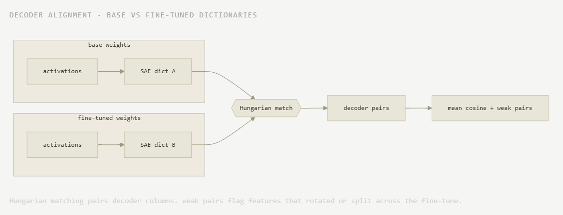
Fine-tuning rotates activation geometry. A dictionary trained on base weights and a dictionary trained on a checkpoint can both reconstruct their respective activations well while assigning completely different indices to what a human would call the same concept. decoder alignment Hungarian-matches decoder columns between two trained SAEs and reports mean cosine similarity plus the weakest pairs.

Alignment is for translation between dictionaries, not for proving quality. A low mean cosine after a large fine-tune is informative: the feature basis moved. It does not mean the temp dictionary failed. Run InterpScore and sae-stats on the checkpoint-trained dictionary before deciding whether to steer with it.

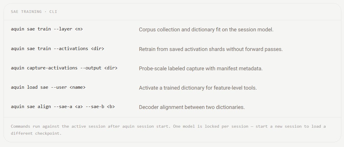
Training is step one of a longer interpretability loop. Collect enough diverse activations that the dictionary can specialize. Watch reconstruction and dead-feature rate during the fit. Load the result and benchmark feature health before building circuits on top. If you fine-tuned the base model, align against a public dictionary only when you need index correspondence, not as a quality gate.

The Attribution article covers what to do once a dictionary is loaded. Benchmarks covers InterpScore, purity, and MUI for deciding which features to trust. Training monitor explains why checkpoint SAE diff often motivates training a new dictionary on fine-tuned weights in the first place.