Simulating Training

Answering the question "what would happen if I trained?" before a single GPU cycle is committed.

Here is the problem with fine-tuning: you find out what went wrong after you paid for it. Your dataset had three poisoned samples that the model happily learned from. Two layers were already dead before training started and accumulated zero gradient throughout. Your learning rate was slightly too aggressive for the landscape curvature at layer 12. You find all of this out when you inspect the checkpoint, which means you already spent the compute.

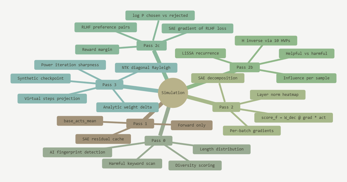
The simulation inverts the whole thing. It reads the actual curvature of the loss landscape before moving any weight. The Neural Tangent Kernel diagonal tells you how much each parameter would move under training. LiSSA approximates the inverse Hessian in linear time and scores every training sample by how much it helps or hurts test generalisation. SAE gradient decomposition projects the gradient onto interpretable feature directions and predicts, by name, which concepts would strengthen and which would be suppressed. All of this before a single optimiser step runs.

The output is not a report. It is a synthetic checkpoint: real PyTorch weights, shifted analytically by the NTK-linearised delta, saved to disk in the same format as a real fine-tune. The SAE diff pipeline, model diff pipeline, behavioral scoring, calibration and all of it runs on the synthetic checkpoint unchanged. The inspection system cannot tell the difference, because structurally there is none.

Most fine-tuning iterations are exploratory. You are not training a production model, you are testing a hypothesis: will this dataset teach the model what I need it to learn? Committing GPU time to a hypothesis test is expensive and slow. The simulation answers the same hypothesis in a fraction of the time, with one critical advantage: it tells you things a real training run cannot.

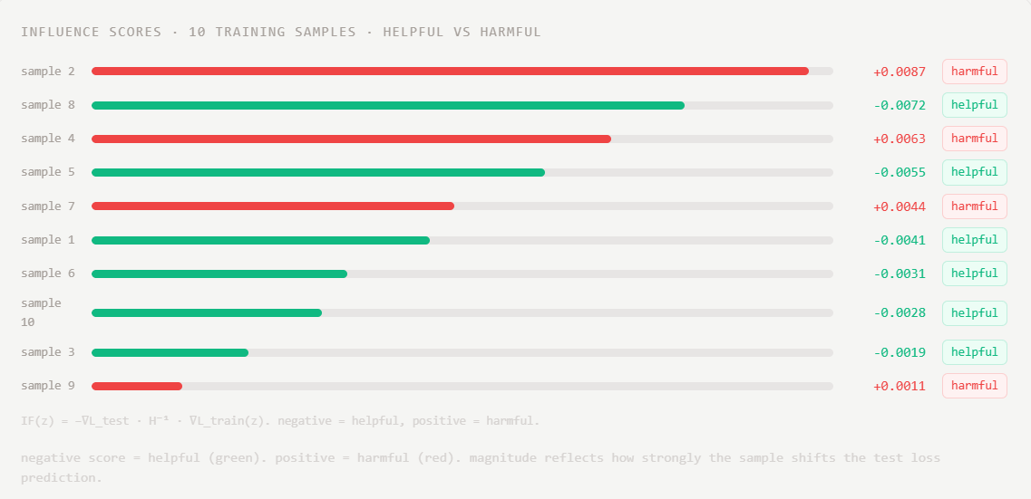
Influence scoring is the clearest example. To know which of your training samples are actively hurting generalisation, you would normally need to retrain with each sample held out and compare the resulting checkpoints. LiSSA does this analytically in a single pass. You get a ranked list of harmful samples before training starts, and you can remove them, re-simulate, and confirm the prediction improved, all without touching a training loop.

The simulation does not replace training. It replaces the first three or four exploratory runs, the ones you were going to throw away once you understood what your data actually contained.

Pass 0 runs without loading the model at all. It analyses the raw dataset text in under a second and answers three questions that decide whether the rest of the simulation is worth running. First: does the dataset contain harmful content? Keyword detection scans every instruction and response field and flags anything that matches. Second: is the dataset contaminated with AI-generated assistant-speak? Phrases like “certainly!”, “as an AI language model”, and “I’d be happy to help” are fingerprints of synthetic data that trains the model to hedge and defer rather than to know things. Third: is the data structurally usable? Length distribution, sequence length violations, and instruction diversity all surface here.

The diversity check is worth lingering on. A dataset with 64 samples that are all slight paraphrases of the same instruction will produce a model that knows one thing very confidently and nothing else at all. The mean pairwise token overlap score quantifies this before you train. A score near 1.0 is a red flag that is invisible from sample count alone.

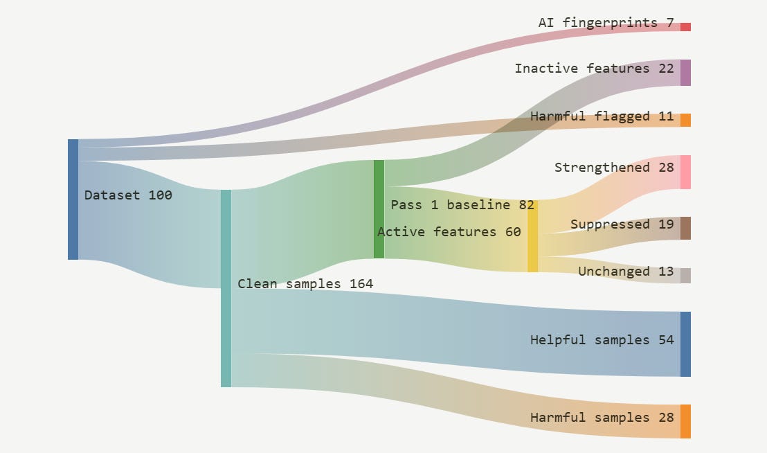
Pass 1 is a forward-only pass with no gradients. It answers one question: which SAE features are already active for this kind of input? The model runs with a residual stream cache at the SAE layer, the SAE encoder maps each activation to a sparse coefficient vector, and the mean across all probe texts becomes base_acts_mean: a vector of shape [n_features] where each entry tells you how active that concept currently is for your dataset.

This baseline is not optional context for Pass 2. It is load-bearing. The SAE gradient decomposition weights every feature’s predicted score by its baseline activation. A feature the model has never used for these inputs gets zero weight regardless of how strongly the gradient aligns with its decoder direction. Predicting that a dormant feature will strengthen because the gradient points at it is like predicting that a muscle will grow because you thought about it. The baseline catches that and zeroes it out.

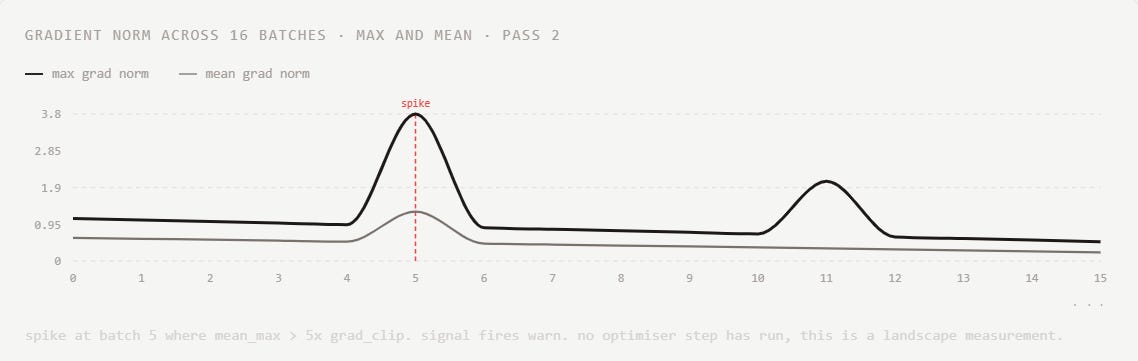
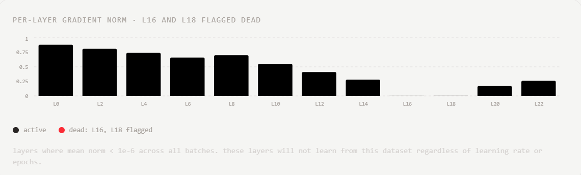
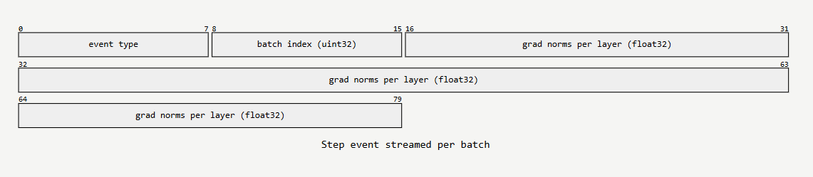
Pass 2 is where training would normally happen, and deliberately does not. A forward and backward pass runs on each batch. The gradients are read, per-layer norms are computed and streamed as live heatmap events, and the global max gradient norm is recorded. No optimiser step is applied. The gradients are pure measurement: they tell you the shape of the landscape your weights sit in.

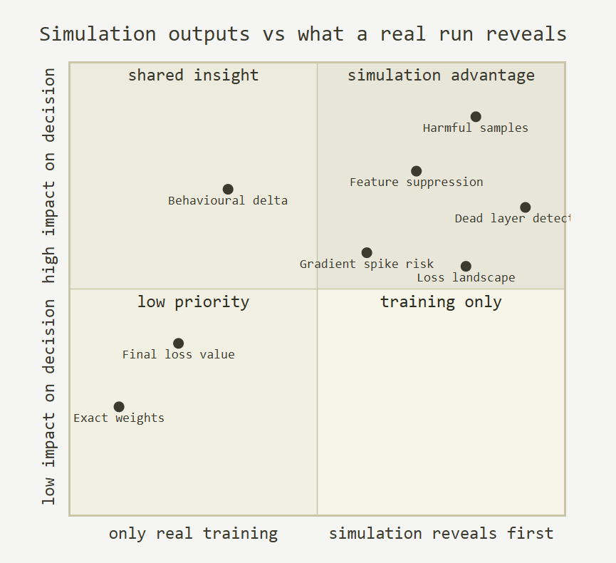
Dead layers show up here in a way that real training hides. In a real training run you might not notice that L16 and L18 have near-zero gradient until you inspect the checkpoint and wonder why those layers look identical to the base model. The simulation surfaces it immediately, before training, as a property of how your dataset activates the network. Those layers have nothing to learn from your data. That is a signal about the data, not about the training procedure.

Gradient spike predictions work the same way. If the mean max gradient across your batches already exceeds 5× grad_clip without any momentum buildup, you will almost certainly see real spikes once Adam’s moment estimates start amplifying. The simulation catches this before the first optimiser step ever runs.

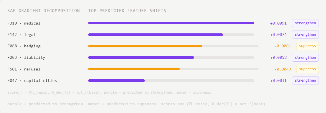
After all batches complete, the mean gradient across the residual stream at the SAE layer is computed. This is where the prediction becomes interpretable. Instead of reporting “the gradient norm at layer 8 is 0.71”, the decomposition asks: which named concepts does that gradient point toward? Each SAE feature has a decoder direction in the residual stream space. The inner product of the loss gradient with that direction tells you how much training pressure is pushing the model toward or away from that concept. Weight the result by the feature’s baseline activation from Pass 1 and you have a per-feature score: how much would this concept shift if training ran to completion.

Features with large positive scores are predicted to activate more strongly after training. Features with large negative scores are predicted to suppress. This is grounded in the actual gradient direction and the actual baseline activations. When F501 (refusal / safety language) shows up with a large negative score on a dataset that contains no refusal content, that is worth investigating before training because it means your data is pulling the model’s safety behaviour in an unexpected direction.

This is the pass that has no equivalent in a standard training loop. Influence functions ask: if I removed this one training sample, how would the model’s test-set loss change? A sample that reduces test loss is helpful, it is genuinely teaching the model something transferable. A sample that increases test loss is harmful, it is teaching the model something that actively hurts generalisation, whether that is an outlier, a mislabelled example, or a sample that reinforces a spurious correlation.

Computing influence exactly requires the inverse Hessian, H⁻¹. For a model with n parameters that is an n×n matrix, hundreds of billions of entries for even a small LLM. LiSSA sidesteps the materialisation entirely by approximating H⁻¹·v via a short iterative recurrence that only ever calls the Hessian-vector product primitive. One LiSSA run computes the inverse-HVP once, then the influence of every training sample is just a dot product against that shared result. The whole pass scales as O(n) in time and O(n) in memory.

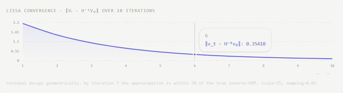
LiSSA is a Neumann series approximation. The key recurrence seeds with the test gradient, then iteratively refines the estimate of H⁻¹·v by applying the Hessian-vector product at each step and folding the result back in with a damping and scale correction. After ten iterations it has converged to a close approximation of the true inverse-HVP without ever materialising the Hessian itself.

Each iteration is one forward pass and two backward passes. Ten iterations total, the only compute cost is twenty backward passes on a single sample. The convergence chart shows the residual dropping geometrically: by iteration 7 the approximation is within 5% of the true H⁻¹v₀. Damping λ=0.01 stabilises convergence when the landscape is flat. Scale s=25 prevents divergence in sharp regions. Both are conservative priors that hold across transformer architectures without tuning.

Preference alignment adds a different objective on top of standard SFT: the model should assign higher probability to chosen responses than to rejected ones. Pass 2c simulates this without running RLHF training by computing the reward margin directly from the current checkpoint. For each preference pair (prompt, chosen, rejected), the model computes log P(chosen | prompt) and log P(rejected | prompt) and takes the difference.

The DPO loss is −log σ(β·margin). The gradient of that loss with respect to the residual stream at the SAE layer is decomposed using the same SAE projection as Pass 2, producing a feature-level view of what RLHF alignment would reinforce and suppress relative to standard SFT. If F501 (refusal / safety) appears in the top reinforced features on a dataset where you did not intend to tune refusal behaviour, the preference labels are driving an unintended alignment.

The mean reward margin at the start of training tells you how hard the alignment phase will have to work. A negative mean margin means the base model actively prefers the rejected responses, the model is aligned backwards and RLHF training will fight the base distribution for every preference pair. That is expensive and often unstable. Knowing this before training starts means you can fix the preference labels or adjust β rather than discovering the instability mid-run.

This is the pass that produces the synthetic checkpoint. It applies the weight changes that T virtual training steps would have produced, analytically, without running any of them. The key insight from the Neural Tangent Kernel theory is that in the linearised regime, every parameter moves in proportion to its gradient and inversely in proportion to the curvature it faces. Parameters in flat regions move far. Parameters in sharp regions move cautiously. The exact formula is:

The weight delta for each parameter is: learning rate times the number of virtual steps, divided by the NTK diagonal entry plus a small damping constant, times the mean gradient for that parameter. Parameters facing high curvature get a smaller effective learning rate. Parameters in flat regions get a larger one. No optimiser loop runs and the delta is applied analytically in a single no-gradient pass and gradient clipping guards against runaway values on dead layers before anything is written to the weights.

Computing the full NTK diagonal exactly would require one Hessian column per parameter, storing it would cost as much as the model itself. The Rayleigh quotient approximation gets the same information from exactly one HVP call per parameter, in the gradient direction:

The Rayleigh quotient measures how much the Hessian amplifies the gradient: how sharply the loss curves in exactly the direction the parameter wants to move. A large K_ii means the loss is steep in that direction; the effective learning rate shrinks and the parameter moves cautiously. A small K_ii means the landscape is flat in the gradient direction; the parameter gets a large effective learning rate and moves aggressively. Dead layers have K_ii near zero, they would receive a runaway effective learning rate but the grad_clip guard catches and rescales the delta before application.

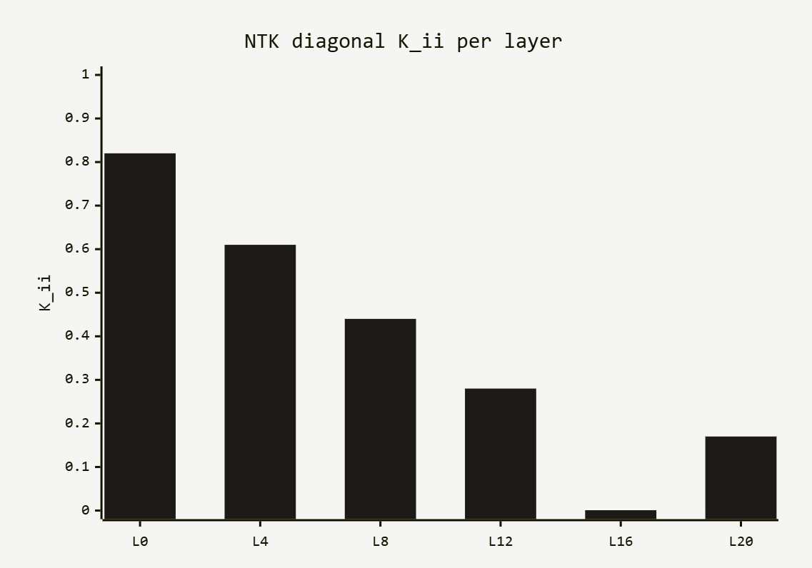
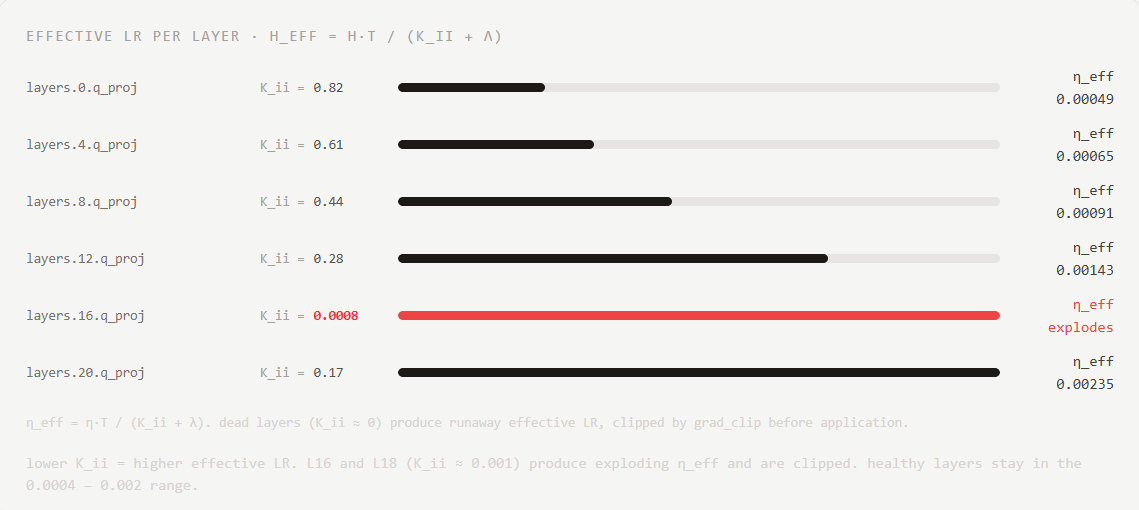
Sharpness is the single number that tells you how reliable the NTK prediction is. The loss landscape is only well-approximated by its linearisation in flat regions. Sharp regions, where the Hessian’s largest eigenvalue is large, are where the linear approximation breaks down fastest as the weights move. power iteration estimates λ_max in three HVP calls:

A sharp landscape (λ_max > 10) means the NTK-linearised predictions are least reliable: the linearisation approximation breaks down where curvature is high. Aquin surfaces this as a sharpness label alongside the effective LR map, so you can judge how much to trust the delta prediction before committing to a real run.

Pass 3 ends with a merge. The LoRA adapter matrices are merged into the base weights and the result is saved to disk. The file is a standard model checkpoint: same keys, same dtypes, same tensor shapes as any real fine-tune you would produce from an actual training run.

This design choice is the entire point. By producing a real checkpoint instead of a structured report, the simulation gains access to every downstream tool in the inspection system without modification. The SAE diff loads base and synthetic checkpoint, runs both through the SAE encoder, and computes the feature-level diff. The model diff runs behavioral scoring on the synthetic checkpoint exactly as it does for real fine-tunes. Circuit tracing, the feature browser, calibration, regression tracking, all of it runs unchanged, because the checkpoint is indistinguishable from the real thing.

The alternative, a structured report that downstream tools would need to parse and adapt to, would have required every inspection tool to add a “simulation mode”. The synthetic checkpoint means zero adaptation. The full power of Aquin’s inspection pipeline is available on a run that committed zero GPU training cycles.

The simulation emits the exact same signal event types as a live training run. Dead layer signals fire when Pass 2 finds layers with mean gradient norm below 1e-6. Gradient spike signals fire when the mean max gradient exceeds 5× grad_clip. The dashboard renders them identically to real training signals, in the same positions in the event stream, with the same severity levels.

The difference is in how you act on them. A dead layer signal from a real training run means stop and investigate the current checkpoint. The same signal from the simulation means this configuration would have produced a dead layer, fix it before you train. Simulation signals are forward-looking warnings, not reports of something that already happened.

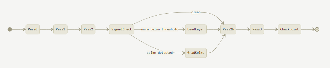
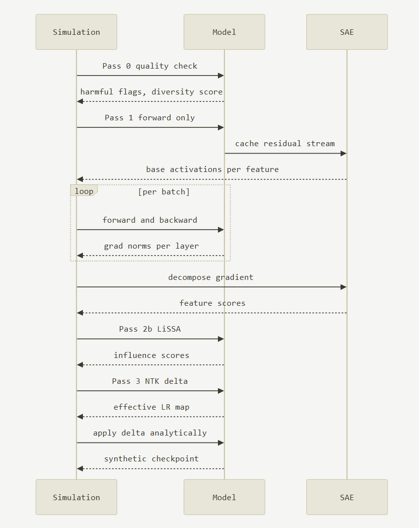
The four passes are a strict dependency chain. Pass 1 needs the model loaded. Pass 2 needs the baseline SAE activations from Pass 1 to weight the gradient decomposition. Pass 2b needs the gradient computations from Pass 2. Pass 3 needs the mean gradients accumulated across all of Pass 2. After Pass 3 writes the checkpoint, SAE diff and model diff run in parallel, the only genuinely concurrent step in the whole pipeline.

The simulation also supports a comparison mode that diffs two saved results side by side: influence score changes between dataset versions, feature score shifts when the training objective changes, effective LR map deltas when learning rate or epoch count is adjusted. The pattern is: simulate, read the harmful samples, remove them, simulate again, compare. By the time you commit to real training you have already seen two or three predicted checkpoints and know which one is worth running.

The git graph below shows exactly this workflow. Simulation v1 flags L16 and L18 as dead and identifies three harmful samples. The dataset is cleaned. Simulation v2 runs clean, surfaces a sharpness warning that prompts a learning rate adjustment. Only then does the real training run commit. The GPU time runs on a configuration that has already been vetted analytically.

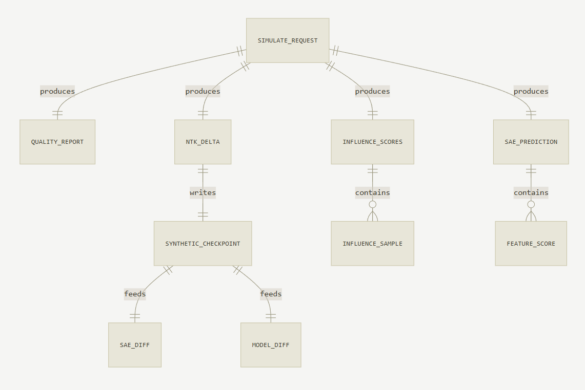
Every simulation produces four first-class artifacts: a quality report, an SAE prediction with per-feature scores, a ranked influence score list, and the synthetic checkpoint itself. They are independent once produced. You can re-run the influence analysis against a cleaned dataset without re-running the gradient passes, or load the synthetic checkpoint in the model inspector without ever touching the original simulation again.

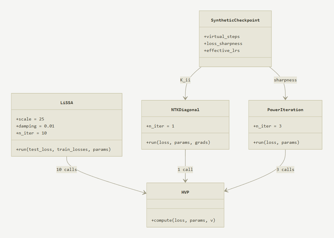
The Hessian-vector product is the primitive everything else is built on. LiSSA calls it ten times to approximate the inverse Hessian. The NTK diagonal calls it once per parameter in the gradient direction. power iteration calls it three times to estimate sharpness. Each call costs one extra backward pass. No Hessian matrix is ever stored.

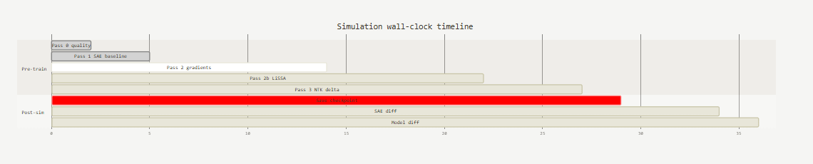
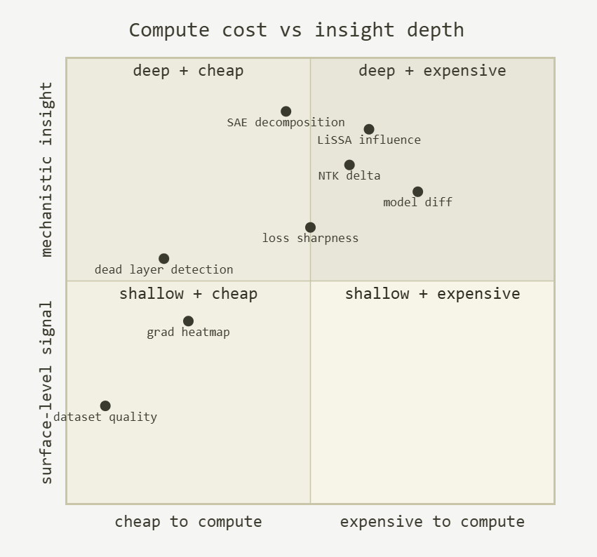
Pass 2 dominates wall-clock time because it runs a full forward and backward pass on every batch. LiSSA adds twenty more backward passes on top of that. Pass 3 is cheap, a handful of HVP calls and a single no-gradient write. The post-sim phase is where the real inspection value unlocks: SAE diff and model diff run in parallel the moment the checkpoint is saved, and everything downstream is available within minutes of the simulation completing.

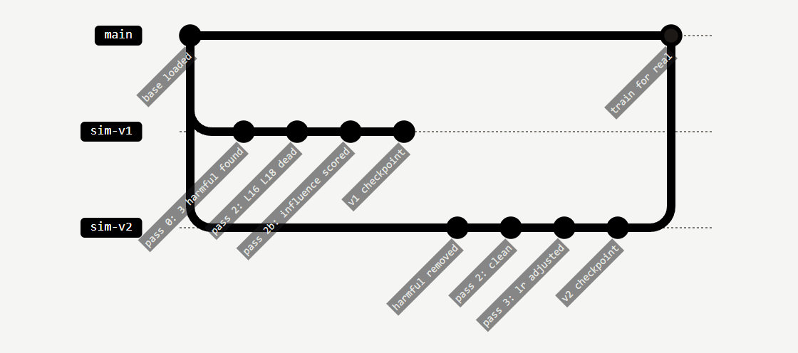
The compare endpoint makes this iterative loop explicit. Diff two simulation results and you see exactly what changed: which samples flipped from harmful to helpful after cleaning, which features shifted when the training objective changed, how the effective LR map moved when the learning rate was adjusted. The pattern is simulate, read, clean, simulate again, compare until the predicted checkpoint is one you would be comfortable shipping.

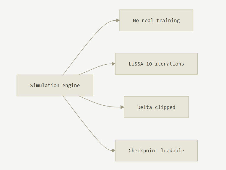
Four invariants hold across every simulation run regardless of model, dataset, or configuration. No gradient-descent loop runs. LiSSA completes within its iteration budget. The NTK-linearised delta is clipped before application. The synthetic checkpoint is a valid state dict loadable by the inspection pipeline. These are not soft guidelines, they are enforced in the implementation and the simulation fails loudly if any of them break.

The simulation answers one question: should I train? By the time it completes you know whether your dataset is clean, which samples are pulling against generalisation, which named concepts the training would strengthen or suppress, whether any layers are dead for your specific data, and what the resulting checkpoint would look like to every downstream inspection tool. That is more than you would know after a real training run, because real training does not score your samples by influence.

If the prediction looks good, commit the compute. If it surfaces harmful samples, remove them and re-simulate. If dead layers appear, investigate whether the data’s coverage of those layers is sufficient. If the sharpness is high, pull the learning rate down and check the effective LR map before the delta blows up on a specific layer. The GPU budget runs on a configuration you have already stress-tested analytically, not a hope.