Using AI to create a magic trick

I recently had my first experience with an LLM solving a seemingly open problem. I wrote about this problem last November, in the form of a proposed card trick presented by a magician with an assistant:

With the magician’s back turned, a spectator thoroughly shuffles a deck of n=52 cards, selects any m=27 (or more) of them, and arranges them face-up in a row left to right, in any desired order. The magician’s assistant flips one of the cards face-down, leaving the spectator’s ordered arrangement otherwise undisturbed. The magician turns around, observes this arrangement with the k=m-1 face-up cards shown, and announces the face-down card(s).

The linked article discusses this trick as another way to generalize Fitch Cheney’s five-card trick. In this case, it’s not difficult to show that the trick is feasible– in principle— if and only if

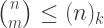
(n)_m \leq (n)_k {m \choose k}

That is, we know the conditions under which there exists an invertible function mapping the set of m-arrangements of cards that the spectator might present to the assistant, into the set of such arrangements with only k cards face-up, that the assistant might “communicate” to the magician.

However, the challenge was to convert principle into practice: is there a practical scheme for performing this trick, ideally computable within the human minds of the assistant and magician, but at the very least simply and efficiently on a computer?

Try as I might, I could not come up with such a scheme. Last December, I asked the humans at MathOverflow for help, including extending the life of the question with a bounty, also with no results.

I also tried to get some insight into this problem from LLMs, primarily the various releases of GPT and Claude. Over the past few years, my personal experiences with “math-heavy” or “algorithmically dense” coding tasks have mostly ranged from amusing to disappointing. This card trick was no different, with agentic code solutions that didn’t work, and comments that were confidently incorrect, but just as exuberantly promising a fix when presented with flaws.

But things have changed since late last year, and for this particular problem, just last month, when Claude Opus 5 solved the problem, at least in part, not only providing a scheme for the trick that could be performed by humans, along with code demonstrating how it works, but also pointing out a key property of the problem that I missed entirely, that seems disturbingly simple in hindsight.

The Python code below demonstrates the trick, with the function acting as both the assistant (assistant=True) and as the magician (assistant=False). In both cases, the idea is to assign +1 to each visible face-up card, -1 to each other card in the deck, and compute the minimum of the sequence of cumulative sums of these {+1,-1} values over some natural ordering of cards in the deck. The assistant flips face-down the card after the last of these minimum value(s) in the sequence, while the magician announces the card at the first minimum.

def fitch_variant(cards: list[int], n: int, assistant: bool):
    """Return hidden card in given list from deck in range(n)."""
    s, s_min = 0, 0
    card_min = -1
    for card in range(n):
        s += (1 if card in cards else -1)
        if s < s_min + int(assistant):
            s_min = s
            card_min = card
    return card_min + int(assistant)

if __name__ == '__main__':
    import random
    n, m = 52, 27
    deck = range(n)
    print('Spectator selects', cards := random.sample(deck, m))
    print('Assistant flips', target := fitch_variant(cards, n, True))
    cards[cards.index(target)] = -1
    print('Magician announces', fitch_variant(cards, n, False))

I say the problem is only solved “in part” because the above only works when k=m-1, that is, when the assistant flips a single card face-down. For example, in principle the spectator could arrange 32 or more cards face-up, two of which the assistant could flip face-down to be announced by the magician. It remains open whether there is a simple and efficient algorithm for doing so.

But this special case of k=m-1 is particularly nice, since the feasibility condition simplifies to 2m>n … which is the same feasibility condition for the admittedly much less interesting trick where the order of the cards doesn’t matter. That is, the Python code above effectively ignores the arrangement of the cards and the position of the “hidden” card in the arrangement. It is as if the spectator presents an unordered subset of m cards to the assistant, who rather than flipping a card face-down, may as well simply remove it altogether, to be announced by the magician.

Alice and Bob on Two-Pi Day

This weekend 6/28 is “Two-Pi Day” (or Tau Day, if you like). Continuing to be on the lookout for surprising or unexpected occurrences of \pi, this year I didn’t have to look farther than an interesting paper by Grimmett [2] in last month’s American Mathematical Monthly.

Suppose that Alice offers Bob the following wager: a fair coin is flipped n=100 times. Alice receives a point for every occurrence of a consecutive pair of heads (HH), while Bob receives a point for every occurrence of heads followed immediately by tails (HT). The player with the most points wins a dollar from the loser. Should Bob take the bet? What is his expected return?

We’ve discussed this game several times here before, most recently calculating the exact expected return, with the perhaps-unintuitive result that Bob has an advantage for any n>2 flips. This is a special case of a more general game where, for each “streak” of s=1 consecutive heads, Alice receives a point for an immediately subsequent “streak-extending” heads, and Bob receives a point for a “streak-ending” tails. We previously presented this more general game in the context of the gambler’s fallacy, where Bob has a roughly 15% advantage when s=4.

The s=3 case was investigated in 1985 by Gilovich, Vallone, and Tversky in [1], looking for evidence of the “hot hand” phenomenon in basketball. They found no significant increase in proportion of “streak-extending” shots made, concluding that a past streak has no effect on current success. However, they seem not to have accounted for this unintuitive unfairness of Alice and Bob’s game. Miller and Sanjurjo in [3] revisit their analysis, arguing that the absence of a bias toward streak-ending missed shots– that we should expect if shots were truly independent but limited in number as with Alice and Bob– suggests that the hot hand is not just “a cognitive illusion.”

So what does all of this have to do with \pi? In [2], Grimmett shows that (for the s=1 game) Bob’s expected return is very well approximated by 1/\sqrt{4\pi n}, and the probability that Alice and Bob tie is asymptotically 1/\sqrt{\pi n}.

References:

  1. Gilovich, T., Vallone, R., and Tversky, A., The Hot Hand in Basketball: On the Misperception of Random Sequences, Cognitive Psychology17(3) July 1985, p. 295-314 [PDF]
  2. Grimmett, G. R., Alice and Bob on X: Reversal, Coupling, Renewal, The American Mathematical Monthly, 133(5), May 2025, 439–451. [arXiv]
  3. Miller, Joshua B. and Sanjurjo, Adam, Surprised by the Hot Hand Fallacy? A Truth in the Law of Small Numbers, Econometrica86(6) November 2018, p. 2019-2047 [arXiv]

Comments on: What Every Experimenter Must Know About Randomization

Introduction

T. Kelly writes in [1] about “What Every Experimenter Must Know About Randomization.” In a running example scenario throughout the paper, Kelly describes a hypothetical poultry farmer who, wondering whether exposing his turkeys to television will fatten them up, conducts a test using N turkey subjects, from which N/2 are randomly selected to receive the TV treatment, with the remaining N/2 control turkeys getting no screen time.

How should the farmer randomize the assignment of turkeys to the treatment and control groups? The main point of the paper– very subtly emphasized in underlined, bold italics– is to “never use a PRNG [pseudo-random number generator] for random assignment.

I don’t really agree with this guidance at all. I think the arguments presented in its favor are flawed, or at least potentially misleading, on practical, mathematical, and even philosophical grounds. But the paper does present at least one very interesting and subtle observation that I think deserves highlighting and clarification.

Balls into bins

To make the case against using a pseudo-random number generator, Kelly provides a C program, balls_into_bins.c, that simulates the random partition of N=32 turkeys into two groups of 16, with one group receiving the treatment and the other being the control group. If we start with all 32 turkeys arranged in a fixed initial order, then uniformly randomly shuffle them, we can designate the leftmost 16 turkeys in the treatment group, and the rightmost 16 turkeys in the control group.

(We don’t actually have to shuffle all 32 turkeys; once we have selected the treatment group– in a uniformly random order– we don’t need to continue rearranging the control turkeys. That is, Kelly effectively implements the first 16 iterations of the mirror_shuffle version of the Fisher-Yates shuffle.)

Kelly’s program then iterates over all 2^{32} possible seeds of the C standard library random number generator via srand(seed), executing this simulated random assignment once for each seed. The idea is to show the distribution of possible assignments, assuming that our farmer conducts the experiment by selecting a “true random” value used as the seed for the PRNG to then (pseudo)randomly shuffle the turkeys to select an assignment.

For a 32-bit seed and N=32 turkeys, these numbers are small enough that we can manage both the time to simulate each seed (i.e., each “ball”), as well as the memory to track all {32 \choose 16}=601,080,390 possible treatment assignments (i.e., “bins”), recording how many times each assignment is selected (i.e., how many balls end up in each bin). Kelly’s results are shown in red in the figure below, indicating the number of bins containing a given number of balls.

For example, the red point at (28,1) indicates that there was a single assignment that was generated 28 times by each of 28 different random seeds. The red point at (0,474467), on the other hand, indicates that 474,467 assignments were never generated, never appearing even once among all 2^{32} possible seeded treatment selections. As Kelly writes:

The resulting distribution of balls into bins will be far from uniform: Some bins end up with more balls than others, and some bins end up empty— even, perhaps surprisingly, when the number of balls is considerably larger than the number of bins.

That is, there are 2^{32}/{32 \choose 16} \approx 7.1 times as many balls as bins, so that the presumably ideal behavior would instead be to distribute the balls as evenly as possible, so that every one of the possible assignments would be selected 7 or 8 times.

Comparing generators

There is a useful point here, which we’ll get to shortly. But first, it wasn’t clear to me whether Kelly is arguing that the non-uniformity illustrated above is because we are using a PRNG. That is certainly not the case… but at the same time, some PRNGs are better than others, and at first glance it seemed like a rather disingenuous straw man to use the one PRNG that most everyone agrees shouldn’t be used “for serious random number generation needs,” namely the one in the C standard library.

For example, how do things look if we try this experiment on Windows, using the MSVCRT/UCRT implementation of rand()? This took some work, since Kelly’s code does not compile due to lines like this:

static_assert(RAND_MAX == INT_MAX); // would be very weird otherwise

This assertion is, well, weird. Not only is there no language standard guarantee that these constants be equal– and on Windows, they aren’t– neither is there anything in the code that depends on this assertion, so it’s unclear why it’s there in the first place.

The program also uses the stdc_count_ones function defined in the stdbit.h header, which is new enough that it may not be available depending on how up to date your environment is, on either Linux or Windows. But here as well, we don’t really need this function, or even an equivalent replacement, to get the job done.

So to get things working, I wrote balls_into_bins.cpp (code is on GitHub, where I’ve included Kelly’s original balls_into_bins.c for side-by-side comparison), with the same behavior, but which (1) works on both Linux and Windows, and (2) allows us to select which of several random number generation approaches we want to evaluate:

  • The Linux GLIBC pseudo-random generator that reproduces Kelly’s original results exactly.
  • The Windows MSVCRT/UCRT pseudo-random generator.
  • The “true” random RDSEED hardware-based generator using the _rdseed64_step function.

The hardware random number generator is understandably much slower; on my laptop it produces only a little over half a million 64-bit words per second. But eventually we see the output shown in blue above, with “non-uniform” behavior very similar to the GLIBC PRNG.

In other words, we should expect to see some treatment assignments selected more often than others. And we should expect to see some assignments not selected at all; with s=2^{32} seeds (“balls”) and r={32 \choose 16} possible assignments (“bins”), the expected number of empty bins is

r(1-\frac{1}{r})^s \approx r e^{-\frac{s}{r}} \approx 473936

which matches pretty closely with the 474,467 empty bins using the GLIBC generator, and the 473,435 empty bins from my particular output using RDSEED.

However, there is clearly something different going on with the Windows UCRT implementation, shown in green above. One interesting “feature” of the UCRT behavior is that we only see even numbers. That is, each assignment (“bin”) is always randomly generated an even number of times– possibly zero times, or twice, or four times, etc., but never exactly once, nor exactly thrice, etc. (Obligatory puzzle: why?)

Repeatability

So what, exactly, is the point being made here? Certainly a poor PRNG like the Windows UCRT generator can cause unintended bias. But the GLIBC PRNG is better behaved, at least from the perspective of the balls-into-bins experiment described here. For example, for both the GLIBC output as well as the “true” random RDSEED output, a chi-squared test would fail to reject the null hypothesis that the selected assignments constitute a truly (uniformly) random sample.

However, there is a key difference between the two generators, namely their repeatability. That is, although it’s true that the RDSEED hardware random generator “misses” nearly half a million possible turkey treatment assignments in the above output, if we were to run the program again with the RDSEED generator, we would once again fail to select roughly half a million assignments… but it would be a different subset of missed assignments. But with the GLIBC PRNG, it is the same persistent subset of exactly 474,467 specific assignments that will never be selected, no matter what seed we use, no matter how many times we run the program. For any one of those persistently-missed assignments, the probability that the farmer selects it for his experiment should ideally be 1/{32 \choose 16}, but instead it’s zero.

“True” vs. pseudo-random numbers

I think it’s an interesting question when, and just how much, this matters in any practical sense for many real experimental scenarios. There are certainly scenarios where it can matter— but in this running example of the farmer experimenting on his turkeys, it’s less clear to me what actual problem might arise from what effectively amounts to bootstrapping from a single prior uniformly sampled multiset from the population of treatment assignments.

But if we did want to “fix” our farmer’s methodology, there are at least a couple of simple ways to do so. For example, Kelly’s setup assumes that the farmer starts by generating 32 “truly” random bits with which to seed a pseudo-random number generator. Maybe those seed bits are obtained by repeatedly flipping a fair coin; but if we’re willing to assume access to 32 “truly random” bits to seed the PRNG, then why subsequently bother with the PRNG at all? As Kelly points out, we only need \log_2 {32 \choose 16} \approx 29.2 bits of entropy, so we need on average at most 2 more, or at most 32 coin flips (on average), to select a random integer and unrank it to determine the corresponding assignment, rather than wasting a lot more coin flips Fisher-Yates shuffling turkeys around.

The above alternative abandons pseudo-random numbers altogether, and only uses a “true” random source of numbers to generate an assignment. I’ve been putting “true” in quotes here, since Kelly never defines or explains exactly what is meant by “true” randomness. It doesn’t seem to require anything quantum mechanical or otherwise theoretical, for example; indeed, the requirements seem pretty lax:

Random assignment does not require a computer. Physical coins or urns are reasonable options sanctioned by many statisticians today, for the same reasons that casinos and lotteries continue to use dice, roulette wheels, and other mechanical contraptions.

Kelly is even okay with “re-using” randomness for an experiment, as long as it’s “unrelated” to that past use:

Regarding “canned” entropy (e.g., from an old-fashioned table of random numbers), I’m aware of no reason why such entropy would lose its usefulness merely from being recorded and stored for a period of time. Similarly, regarding “recycled” entropy that has already been used for purposes unrelated to the one at hand, I’m aware of no reason why such entropy would be any less useful than if it had not been used before for any purpose.

This is what I find confusing and contradictory. A not-completely-terrible intuitive description of a PRNG is “an old-fashioned table of random numbers”… but one that is so large that we never need to re-use any of it. That is, for example, suppose that when we complete our undergraduate statistics education, we seed a pseudo-random number generator, one time, and use that single stream of random numbers for the duration of our lifetime, or at least for our entire career as an experimenter. When we need some random numbers, we extract them, then store the subsequent generator state on disk. When we need some more random numbers, we restore the generator state from disk, extract some more random numbers, rinse and repeat.

If our experiments are “slow” like testing turkeys, and not “fast” like computer simulations, then such a single pseudo-random stream is plenty long enough to support more experiments on more test subjects than our farmer can possibly conduct in their lifetime. And if we are worried, as Kelly writes, that “the outcome is a foregone conclusion, completely devoid of uncertainty, no matter how random the sequence might appear,” then why is an old-fashioned published book of random numbers acceptable?

Reference:

  1. Kelly, T., What Every Experimenter Must Know About Randomization, ACM Queue Magazine, 23(6), November/December 2025. [PDF]

Analysis of Biscuits dice game

Introduction

In the dice game “Biscuits,” a player rolls 12d6+1d8+1d10+1d12, then selects one or more of the rolled dice to set aside, rolling the remainder again, continuing this process until eventually all 15 dice have been set aside. The player’s score is the sum of the final values shown on the dice, with the highest score winning the game.

A rolled six on a d6– or an eight on the d8, or generally the maximum value on a die– is referred to as a biscuit… and as the rules suggest, “you want biscuits and lots of them!”, where “sometimes you’ll roll several biscuits all at once, you can set them all aside.”

You can set them all aside… but should you? That is, suppose that you roll sixes on multiple d6s at once, but relatively small values for the d8, d10, and/or d12. Should you set aside all of those biscuits, banking the highest possible score for those dice, or is it worth it to “give up” some of that guaranteed score in exchange for more future opportunities to roll better scores for the d8, d10, and d12?

Results

Not to beat around the bush, the latter turns out to be the case. Strategy in this game appears to be pretty interesting; let’s suppose that our objective is to maximize our expected total score (more on this later). Python code is available on GitHub to evaluate all possible moves that we might make from any given roll. For a most extreme example situation, suppose that on the initial roll we get biscuits for all 12d6, but we roll 1 for each of the other dice:

>>> analyze(((0, 0, 0, 0, 0, 12),
             (1, 0, 0, 0, 0, 0, 0, 0),
             (1, 0, 0, 0, 0, 0, 0, 0, 0, 0),
             (1, 0, 0, 0, 0, 0, 0, 0, 0, 0, 0, 0)))
 93.836 points by keeping d6 (6 ), 
 93.761 points by keeping d6 (6 6 ), 
 93.691 points by keeping d6 (6 6 6 ), 
 93.625 points by keeping d6 (6 6 6 6 ), 
 93.565 points by keeping d6 (6 6 6 6 6 ), 
 93.509 points by keeping d6 (6 6 6 6 6 6 ), 
 93.462 points by keeping d6 (6 6 6 6 6 6 6 ), 
 93.449 points by keeping d6 (6 6 6 6 6 6 6 6 6 6 6 6 ), 
 93.427 points by keeping d6 (6 6 6 6 6 6 6 6 6 6 6 ), 
 93.426 points by keeping d6 (6 6 6 6 6 6 6 6 ), 
 93.407 points by keeping d6 (6 6 6 6 6 6 6 6 6 ), 
 93.407 points by keeping d6 (6 6 6 6 6 6 6 6 6 6 ), 
 87.292 points by keeping d6 (6 6 6 6 6 6 6 6 6 6 6 6 ), d8 (1 ), 
 87.167 points by keeping d6 (6 6 6 6 6 6 6 6 6 6 6 ), d8 (1 ), 
 87.064 points by keeping d8 (1 ), 
 87.037 points by keeping d6 (6 6 6 6 6 6 6 6 6 6 ), d8 (1 ), 
...

Optimal strategy is to keep just a single d6, sacrificing all 11 other biscuits in exchange for more future rolls to hopefully improve the contribution from the d8, d10, and d12. Even more interesting is that the expected total score isn’t monotonic in how many biscuits we might choose to set aside: keeping one d6 is best, and keeping all 12 is worse… but not as bad as keeping just 10 of them.

The figure below shows the distribution of possible total scores using this strategy, sampled from 10,000 simulated games.

Distribution of final total score in Biscuits using expectation-maximizing strategy, with expected score of about 93.9 (out of 102 possible) shown in red.

I was surprised at how well this strategy performs, with an expected score of about 93.9 (shown in red), and in a few simulated games even reaching the maximum possible score of 102.

Implementation

As discussed previously here, we can efficiently enumerate all possible outcomes from rolling a given subset of the dice as weak compositions of the total number of dice of each type. To compute optimal strategy for a given roll, we consider all possible non-empty subsets of dice to keep, recursively evaluating the expected score of each such move, memoizing results as we go.

As an aside, the Python code was not the starting point. Quite often I find it useful to do my “thinking” in Mathematica, then convert the resulting algorithm into a more widely accessible form. It’s always interesting to see how much more concise– but often much less readable– the Mathematica implementation usually is, as shown below.

rolls[n_, d_] := Map[
  Differences[Append[Prepend[#, 0], n + d]] - 1 &,
  Subsets[Range[n + d - 1], {d - 1}]
  ]

score[ns_, ds_] := score[ns, ds] = Total@Map[
  (Times @@ Multinomial @@@ #) Max[0, Map[
    Total[Total /@ (Range[ds] #)] + score[ns - (Total /@ #), ds] &,
    Rest[Tuples[Tuples /@ Range[0, #]]]
    ]] &,
  Tuples[MapThread[rolls, {ns, ds}]]
  ] / Times @@ (ds^ns)

score[{12, 1, 1, 1}, {6, 8, 10, 12}]

Open questions

I think there are a lot of interesting additional questions to pursue here. For example, is there a concise description of optimal strategy, or even an approximation of it, that a human player can implement with simple mental calculation?

Can the calculation of optimal strategy be made more efficient? Interestingly, both the Mathematica and Python implementations took about a day and a half to execute on my laptop. Add any more dice and things would get out of hand.

Finally, the strategy analyzed above is only optimal in the sense of maximizing expected score. This is not the same thing as maximizing the probability of beating another player. Similar to the approach utilized here, ideally we would evaluate the second player’s strategy first, with the utility function parameterized by the first player’s hypothetical final score. Then, once we know all of the possible expected values for the second player, we could compute the first player’s optimal strategy and overall value of the game, using the (negated) second player’s expected returns as the utility function. How different do the resulting strategies look as a result, compared with maximizing expectation?

Analysis of Mastermind-like bottle match game

During the holidays, my niece introduced me to a “bottle match” game, variants of which have apparently made the rounds online for a while now, but it was new to me. She secretly arranges seven wooden bottle-shaped pegs, each of a different color, in a row. I then make a series of guesses of the ordering of the colors (arranging a second set of seven bottles visible to everyone), with each guess scored with a number indicating how many bottles are in the correct position. The objective is to get all seven bottles in the correct order in as few guesses as possible.

This is very similar to the board game Mastermind: one player arranges a secret “code,” and another player makes a series of guesses, with scores providing partial information about how close each guess is to the solution.

Watching family members play the bottle match game, I wondered how inefficient we were being in our guesses. Our exploration of the space of possible solutions seemed pretty timid, making “small” single-transposition changes to the arrangement of bottles at each step, even backtracking to previous guesses at times just to confirm remembered scores.

With n=7 bottles, a coarse lower bound of at least \lceil\log_{n-1}n!\rceil=5 guesses are necessary in the worst case. How close to this bound can we get?

I wrote a program to try to answer this question, taking advantage of the similarity to Mastermind to analyze both games in the process. The resulting ~100 lines of Python code are on GitHub.

The greedy heuristic strategy used for both games is that described by Knuth (2): at each turn, make a guess that minimizes the maximum number of possible secret codes that might remain, over all possible scores that the guess might receive. Break any ties by first preferring codes that are possible (so that we have a chance of winning on the next move)… and in the case of the bottle match game, prefer a code that is “closest” to the previous guess, in the sense of requiring the least amount of additional shifting bottles around to turn the previous guess into the new guess.

This distance metric on permutations can be hard to compute, depending on what sort of shifting operations are allowed. The “block interchange” metric described by Christie (1) seems reasonably realistic for this problem, while being efficiently computable: one operation involves taking two “blocks” of consecutive bottles and swapping them, as shown in the example in the figure below.

Example of a single block interchange operation, swapping the block of 3 bottles in the gray box with the block of 2 bottles in the black box.

As a sanity check, evaluating the resulting strategy for the Mastermind game across all 6^4=1296 possible secret codes, replicates the results in Knuth’s paper: an expected number of guesses of 5801/1296, or about 4.476, never requiring more than a maximum of 5 guesses.

For the bottle match game, we can guess the secret code in 34169/5040, or about 6.78 guesses on average, never requiring more than a maximum of 8 guesses. It’s interesting how often it is advantageous– at least in this greedy heuristic minimax sense– to guess a code that is not consistent with the scores observed so far, as shown in the example output below.

>>> import mastermind
>>> game = mastermind.ColorMatch()
>>> game.play((6, 5, 4, 3, 2, 1, 0), show=True)
Guess (0, 1, 2, 3, 4, 5, 6) in 5040 remaining: score 1
Guess (2, 3, 4, 5, 6, 1, 0) not in 1855 remaining: score 3
Guess (2, 5, 0, 1, 6, 3, 4) not in 106 remaining: score 1
Guess (4, 3, 0, 1, 6, 5, 2) not in 31 remaining: score 0
Guess (2, 1, 4, 5, 0, 3, 6) not in 8 remaining: score 1
Guess (6, 5, 4, 3, 2, 1, 0) in 2 remaining: score 7

References:

  1. Christie, D., Sorting permutations by block-interchanges, Information Processing Letters, 60(4) November 1996, p. 165-169.
  2. Knuth, D., The Computer as Master Mind, Journal of Recreational Mathematics, 9(1) 1976-77.

Riddler Solution: Can You Skillfully Ski The Slopes?

Introduction

In Zach Wissner-Gross’s Fiddler on the Proof, he mentions the following problem from nearly five years ago, when it was still FiveThirtyEight’s The Riddler:

You are one of n=2 finalists in a skiing championship. There are two rounds: in the first round, each finalist skis down the mountain, recording their finishing time; this is repeated in the second round, with the least total time for both runs winning the championship. This is the top talent in the world, so the time for every run is independent and identically distributed. Having learned that you have the best time in the first round, what is the probability that you will win the championship? For extra credit, what if n=30?

In the original problem, the finishing times were normally distributed. The neat feature of this problem is a cocktail-napkin solution for n=2 that does not depend on this distribution. However, the extra credit for larger n— for normally distributed run times– appears to require resorting to simulation or approximation, although Josh Silverman provides some really interesting recent asymptotic analysis.

The motivation for this post is to capture my notes on the exact solution for any n for the case where finishing times are uniformly distributed. (This feels to me like a slightly more natural version of the problem, without the unrealistic negative tails.)

Solution

Define random variables X and Y to be the finishing times for our first and second run, respectively, and similarly define R_i and S_i to be the first and second round times for each competitor i \in \{1,2,\ldots,n-1\}. Define event A_i to be X+Y<R_i+S_i (i.e., we beat competitor i overall) and event B_i to be X<R_i (i.e., we beat competitor i in the first round). Then we want to compute the probability

P(\bigcap\limits_{i=1}^{n-1}A_i | \bigcap\limits_{i=1}^{n-1}B_i)

Applying Bayes’ theorem, and re-ordering and re-grouping the intersection of events in the numerator, we have

\frac{P(\bigcap\limits_{i=1}^{n-1}A_i \cap B_i)}{P(\bigcap\limits_{i=1}^{n-1}B_i)}

There are two key observations: first, by symmetry, the probability in the denominator– that we are the leader after the first round– is 1/n. Second, in the numerator, if we condition on fixed times for our two runs, say for example X=x=0.3 and Y=y=0.8, then the n-1 events A_i \cap B_i are independent– so we can multiply them– and they all have the same probability.

The following figure shows this example situation, where the area of the shaded region is the probability P(A_i \cap B_i)=P(x+y<R_i+S_i \land x<R_i) that we beat a particular competitor in both rounds.

This shaded region has two different shapes depending on whether x+y is less than or greater than 1; putting everything together, the desired probability is

n \int_{x=0}^1(\int_{y=0}^{1-x}(1-x-\frac{1}{2}y^2)^{n-1}\mathrm{d}y + \int_{y=1-x}^1((1-x)(1-y)+\frac{1}{2}(1-x)^2)^{n-1}\mathrm{d}y)\mathrm{d}x

Applying binomial expansion to the powers and moving the integrals inside the resulting summation gives the following formula:

n\sum\limits_{k=0}^{n-1}{n-1 \choose k}\frac{1}{2^k}(\frac{(-1)^k}{(2k+1)(n+1+k)}+\frac{(n-1-k)!(n-1+k)!}{(2n)!})

The figure below shows this probability vs. the number of skiers n.

For 5 or 6 skiers, it’s roughly a coin toss whether you retain your first-round lead. When n=30, the probability is about 0.226.

Variants of Fitch Cheney’s Trick

Nearly 15 years ago, I wrote about the following trick attributed to William “Fitch” Cheney, Jr., in [1]:

Effect 1: While the magician turns their back or even leaves the room, a spectator shuffles a standard deck of n=52 cards, and selects an (unordered) subset of any m=5 cards and hands them to the magician’s assistant. For example:

Cards selected by the spectator.

The assistant arranges k=4 of these cards in a row left to right, as shown below, keeping the remaining selected card hidden.

Cards presented to the magician.

Upon observing this arrangement, the magician announces the fifth selected card, in this case the ace of diamonds.

The article linked above describes how the trick works in practice (including Python source code demonstrating both the assistant and the magician), as well as a proof that the following condition on (n,m,k) is necessary and sufficient for the trick to be feasible, at least in principle:
{n \choose m} \leq (n)_k

Intuitively, the LHS binomial coefficient counts the number of spectator selections that may be presented to the assistant, and the RHS falling factorial counts the number of arrangements that may be presented to the magician.

The motivation for this post is to observe that this basic argument, applying the König-Egerváry theorem to a bi-regular graph to find a saturating matching, is more generally applicable: it should be possible to perform other “Fitch-like” tricks, whose feasibility rests on similar counting arguments. For example:

Effect 2: A spectator rolls m=6 dice each with n=6 sides (maybe from their Farkle set), and arranges the dice in a row left to right, in any desired order. The assistant covers one of the dice by placing a cup over it, leaving the ordered arrangement otherwise undisturbed. The magician observes this arrangement with the k=m-1 values shown, and announces the value on the covered di(c)e.

This trick is feasible if and only if:

n^m \leq n^k {m \choose k}

For another example of this same form, (n,m,k)=(10,10,9) corresponds to writing down a 10-digit number, the assistant covering one of the digits, and the magician announcing the hidden digit.

The linked proof shows that both of these tricks are feasible in principle— but it’s a separately interesting challenge to come up with a practical scheme for performing them. In this case, there is a relatively simple solution left as a puzzle for the reader; but things can get complicated quickly, as in this puzzling.stackexchange.com post that discusses the (6,9,7) case.

Effect 3: A spectator selects any m=27 cards from a deck of n=52 cards, and arranges them face-up in a row left to right, in any desired order. (More practically, imagine shuffling and cutting strictly more than half the deck, and fanning the cards face-up in a row.) The assistant flips one of the cards face-down, leaving the ordered arrangement otherwise undisturbed. The magician observes this arrangement with the k=m-1 face-up cards shown, and announces the face-down card(s).

In this case, the trick is feasible if and only if:

(n)_m \leq (n)_k {m \choose k}

Of these two variants, I think this one would be the more powerful effect. Note that unlike Fitch’s original trick, the spectator gets to not only choose the cards, but to arrange them in any chosen order as well. The assistant’s only freedom is in which card(s) to flip face-down.

Here again, the obligatory puzzle is to determine a practical scheme for performing this trick. I’m not sure how much it helps as a hint to note that, in this particular case of k=m-1 where the assistant flips exactly one card face-down, for the trick to be possible we need the spectator to select and arrange strictly more than half of the cards in the deck. (So that, for example, it is perhaps useful that the spectator is guaranteed to select at least one pair of cards of the same rank and color in their arrangement?)

Reference:

  1. Kleber, M., The Best Card Trick. Mathematical Intelligencer24 (2002). [PDF]

The criminal coupon collector

Introduction

Alice and Bob ride their bicycles together to work each day. They each secure their bicycles using chain combination locks with m=6 dials, with 10 decimal digits on each dial.

“I notice you always take longer than I do to lock your bike,” Alice says, “and I spin each of my dials independently and uniformly after locking– making sure I don’t accidentally leave it unlocked. What takes you so long?”

“I spin my dials after locking, too, ” Bob says, “but I also make sure that none of the individual dials on the lock happens to be correct, giving it extra random spins if necessary. No sense in helping a thief get lucky.” (In other words, for example, if Bob’s combination is 123456, then he may leave the combination spun to 451234, but not 151234, since the first digit would be correct.)

Eve is the neighborhood thief, who has noticed these two expensive-looking bicycles at this same location every morning for a while now, and she happens to overhear this conversation. After watching Alice and Bob lock their bikes and enter their building, Eve casually strolls over and observes the sequence of digits on each of the locks. She has an idea.

Puzzle 1: Assuming Eve is able to observe the combination on Alice’s lock and try exactly one combination each morning after Alice leaves her bike for work, what is the expected number of days until she is able to steal the bike?

Puzzle 2: Similarly observing the displayed combination on Bob’s lock, what is the expected number of days until Eve is able to steal Bob’s bike?

Multiple coupon collectors

Stealing Alice’s bike is an interesting problem in its own right. But the focus of and motivation for this post is to capture my notes on the second problem of stealing Bob’s bike. The practice of ensuring that none of the individual combination dials is randomly accidentally correct, while well-intentioned, ends up making Eve’s job much easier. Despite the lock having one million possible combinations, Eve needs less than 40 days’ worth of observations on average to steal the bike.

We can rephrase the problem in terms of multiple coupon collectors: there are m collectors, one for each dial, each independently trying to collect s=10-1=9 coupon types, one for each incorrect digit on that dial. Each day, all m collectors draw a coupon; we want to compute the expected number of days until all collectors have each obtained all coupon types. Put another way, we want the expected value of the maximum of m independent random variables, each distributed according to the standard solo coupon collector problem with s coupon types.

The cumulative distribution for this maximum N is

P(N \leq n) = (\sum\limits_{k=0}^s (-1)^k{s \choose k}(1-\frac{k}{s})^n)^m

with expected value

E(N) = -\sum\limits_{\mathbf{k}>\mathbf{0}} \frac{\prod\limits_{i=1}^m (-1)^{k_i}{s \choose k_i}}{1-\prod\limits_{i=1}^m (1-\frac{k_i}{s})}

where the summation ranges over tuples \mathbf{k} of m non-negative integers that are not all zero, corresponding to a number of “unknown incorrect” digits for each dial. In Python:

from fractions import Fraction
from itertools import islice, product
from math import comb, prod

def probability_coupon_draws(n, s, m=1):
    """CDF(# of coupon draws from s types for all of m collectors)."""
    return sum((-1) ** k * comb(s, k) * (1 - Fraction(k, s)) ** n
               for k in range(s + 1)) ** m

def expected_coupon_draws(s, m=1):
    """E(# of coupon draws from s types for all of m collectors)."""
    return -sum(prod((-1) ** k_i * comb(s, k_i) for k_i in k) /
                (1 - prod(1 - Fraction(k_i, s) for k_i in k))
                for k in islice(product(range(s + 1), repeat=m), 1, None))

The result is about 39.5891 observations on average until Eve knows all 9 incorrect digits for each dial, and thus knows the entire correct combination.

Binomial proportion estimation with unknown and varying number of trials

Here is a neat trick: our friend, Paul, has asked us for help estimating his skill at the shooting range. Every day for the past several years, he has diligently recorded the number x_i of successful shots he took that day. Assuming that every shot is an iid Bernoulli trial with success probability p, can we estimate p?

Unfortunately, no. Paul only recorded the number of successful shots each day. If he hit the target x_i=20 times on a given day, was that out of 20 attempts, or 25, or 150? Not only did Paul not record that corresponding total number n_i of attempted trials each day, but that total varied from one day to the next: some days it might be just one “stand” of 25 shots, other days it might be several hours with hundreds of shots.

It might seem like we’re stuck. However, Paul mentions that he doesn’t shoot alone. His friend, Quinn, has accompanied him on each of these trips to the shooting range. In friendly competition, they each take the same number of shots, and whoever has the most hits buys a round on the way home. Fortunately, Quinn has kept a similar record of his daily hits (but again, not daily total trials).

This is interesting: Quinn takes each shot with some different success probability q, that is just as unknown to us as p. How can similarly incomplete information about Quinn possibly help us learn something about Paul?

It turns out that it can; following is Python code implementing a simpler one of several different estimates of Paul’s success probability p, given a list of pairs of Paul’s and Quinn’s hit counts.

def estimate_p(xy: list[tuple[int, int]]) -> float:
    """Estimate Bernoulli probability from pairs of success counts."""
    sx  = sum(x     for x, y in xy)
    sy  = sum(y     for x, y in xy)
    sxy = sum(x * y for x, y in xy)
    sx2 = sum(x * x for x, y in xy)
    return 1 - sx2 / sx + sxy / sy

The figure below shows this estimate vs. Paul’s true success probability, for each of 100 simulated experiments, where we randomly choose true success probabilities for Paul and Quinn.

Simulation of 100 experiments (one point each) with uniformly random p and q, showing resulting estimated vs. true probability p.

Code for these experiments and plotting results is on GitHub.

A trick-taking game

There has not been a puzzle here in a while, so…

Alice is playing a card game with her nephew, Bob, using a standard deck of playing cards. Alice starts with the 26 red cards in her hand, and Bob starts with the 26 black cards in his hand. In each of 26 rounds (or tricks), Alice and Bob simultaneously select and play one card from their remaining hand. The player with the higher-ranked card takes the trick; cards of the same rank are discarded with neither player taking the trick. After all cards have been played, Alice wins (loses) one point for every trick won (lost).

At this point, by symmetry, this seems like a fair game. To skew things slightly in her nephew’s favor, Alice suggests a wrinkle: aces are low… except for one of Bob’s aces, the ace of spades, which is high, ranking higher than all other cards.

  1. What are Alice’s and Bob’s optimal strategies and corresponding expected score in this game?
  2. Suppose that instead of a point for every trick, the player with the most tricks wins the game (with a score of +1, or 0 if both players take the same number of tricks). What are Alice’s and Bob’s optimal strategies and expected score?
  3. How does this generalize to arbitrary initial hands? That is, suppose Alice and Bob start with known card ranks a_1 \leq a_2 \leq \ldots \leq a_n and b_1 \leq b_2 \leq \ldots \leq b_n, respectively (with all cards known to both players).