Frolian's blog standing on the shoulders of PyGiants

• About
• Archive

Understanding the Karplus-Strong with Python (Synthetic Guitar Sounds Included)

Thu, 20 Apr 2017

Music

This post was entirely written using the IPython notebook. Its content is BSD-licensed. You can see a static view or download this notebook with the help of nbviewer at 20170419_KarplusStrongAlgorithm.ipynb.

In this blog post, we will implement the Karplus-Strong algorithm for guitar sound synthesis.

What is the Karplus-Strong algorithm?

The Karplus-Strong algorithm, named after its two creators, was originally published in 1983 as the following paper (full paper here):

Karplus, Kevin, and Alex Strong. “Digital Synthesis of Plucked-String and Drum Timbres.” Computer Music Journal 7, no. 2 (1983): 43–55.

As the paper states, it is a simplified digital instrument that allows one to control pitch, amplitude and decay time. What is so interesting about the algorithm is that it yields realistic sounds even though it is very simple.

How does the algorithm work?

To answer that question, we will first briefly go over how wavetable synthesis works.

Wavetable synthesis

Wavetable synthesis was invented in the 1970's. It is based on the following idea: suppose you have an array of points describing a wave.

%matplotlib inline
import matplotlib.pyplot as plt
import numpy as np

t = np.linspace(0, 1, num=100)
wavetable = np.sin(np.sin(2 * np.pi * t))

plt.plot(t, wavetable, '-o')

[<matplotlib.lines.Line2D at 0x7ddb908>]

What happens if we imagine a pointer going through our wavetable at different speeds and picking the closest point it finds to generate a new waveform with it?

from moviepy.editor import VideoClip
from moviepy.video.io.bindings import mplfig_to_npimage

duration = 2

pointer1 = 1
pointer2 = 2
points1 = []
points2 = []
fig, axes = plt.subplots(2, 1)
def make_frame(time):
    ax = axes[0]
    ax.clear()
    ax.plot(t, wavetable)
    ax.vlines(pointer1 * time / duration, -1, 1, color='red', label='slow pointer')
    ax.vlines(pointer2 * time / duration % 1, -1, 1, color='blue', label='fast pointer')
    for pointer, color, points in zip([pointer1, pointer2], ['red', 'blue'], [points1, points2]):
        arg = np.argmin(np.abs(t - (pointer * time / duration % 1)))
        ax.plot(t[arg], wavetable[arg], 'o', color=color)
        points.append(wavetable[arg])
    ax.set_xlim(0, 1)
    ax.legend(loc='lower left')
    
    ax2 = axes[1]
    ax2.clear()
    ax2.plot(points1, '-or')
    ax2.plot(points2, '-ob')
    ax2.set_xlim(0, 41)
    ax2.set_ylim(-1, 1)
    return mplfig_to_npimage(fig)

animation = VideoClip(make_frame, duration=duration)
plt.close(fig)
animation.ipython_display(fps=20, loop=True, autoplay=True)

 98%|████████████████████████████████████████▉ | 40/41 [00:05<00:00,  6.93it/s]

As we can see from the above diagram, the fast pointer goes trough the waveform twice as fast as the original pointer. However, as it reaches the end of the wave, it starts over at the beginning. Using this method, we can easily derive several new waveforms from the original wavetable by looping over the wavetable and going back to the beginning when we reach the end of the wavetable. Fun fact, this is how a Gameboy generates sounds.

Let's write a function that implements the wavetable synthesis principle.

def synthesize(sampling_speed, wavetable, n_samples):
    """Synthesizes a new waveform from an existing wavetable."""
    samples = []
    current_sample = 0
    while len(samples) < n_samples:
        current_sample += sampling_speed
        current_sample = current_sample % wavetable.size
        samples.append(wavetable[current_sample])
        current_sample += 1
    return np.array(samples)

Let's see what the outputs look like.

sample1 = synthesize(1, wavetable, 300)
sample2 = synthesize(2, wavetable, 300)

plt.plot(sample1)
plt.plot(sample2)
plt.xlabel('sample number')

<matplotlib.text.Text at 0xa6b5908>

What we see is that the waveforms look quite similar except for the fact that one has a higher frequency than the other.

Let's generate some sounds at interesting frequencies. We first generate a new wavetable designed for a sampling rate of $f_s$ = 8000 Hz.

fs = 8000

t = np.linspace(0, 1, num=fs)
wavetable = np.sin(np.sin(2 * np.pi * t))

plt.plot(t, wavetable, '-o')

[<matplotlib.lines.Line2D at 0xaa9e278>]

Now, let's generate a sinusoid at 220 Hz and one at 440 Hz.

sample1 = synthesize(220, wavetable, 2 * fs)
sample2 = synthesize(440, wavetable, 2 * fs)

We can listen to it using the IPython rich output:

from IPython.display import Audio

Audio(sample1, rate=fs)

Audio(sample2, rate=fs)

Indeed the sampling scheme works, sample2 has a higher frequency than sample1.

One of the strenghts of this type of wavetable synthesis is that you can easily move to more complex sounds, with harmonics and still use the same model. For instance, we can use a triangle shape:

wavetable = t * (t < 0.5) + (-(t - 1)) * (t>= 0.5)

plt.plot(t, wavetable, '-o')

[<matplotlib.lines.Line2D at 0xab5b080>]

Again, let's sample two sounds:

sample1 = synthesize(220, wavetable, 2 * fs)
sample2 = synthesize(440, wavetable, 2 * fs)

Audio(sample1, rate=fs)

Audio(sample2, rate=fs)

Or, a more complex sine based wavetable.

def make_sine_wavetable(n_samples, amps, phases, freqs):
    """Makes a wavetable from a sum of sines."""
    t = np.linspace(0, 1, num=n_samples)
    wavetable = np.zeros_like(t)
    for amp, phase, freq in zip(amps, 
                                phases,
                                freqs):
        wavetable += amp * np.sin(np.sin(2 * np.pi * freq * t + phase)) + \
                         amp / 2 * np.sin(np.sin(2 * np.pi * 2 * freq * t + phase))
    return wavetable

wavetable = make_sine_wavetable(t.size, [0.1, 0.5, 0.8, 0.3], 
                            [0, 0.3, 0.4, 0.7],
                            [1, 2.1, 3, 4.3])

plt.plot(t, wavetable, '-o')

[<matplotlib.lines.Line2D at 0xa96a9e8>]

sample1 = synthesize(220, wavetable, 2 * fs)
sample2 = synthesize(440, wavetable, 2 * fs)

Audio(sample1, rate=fs)

Audio(sample2, rate=fs)

Now of course this does not sound like a realistic instrument, for several reasons.

• the wavetable has not the shape of a realistic instrument sound
• there is no dynamic part in the generated sound like attack and decay

Indeed, if we wanted to, we could use more complex wavetables like this one:

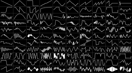
And we could also add some an ADSR (attack, delay, sustain, release) envelope to the waveform.

However, we will skip this here and move on to the Karplus-Strong algorithm.

Changing the wavetable: the Karplus-Strong algorithm

As explained in the original article:

The wavetable-synthesis technique is very simple but rather dull musically, since it produces purely periodic tones. Traditional musical instruments produce sounds that vary with time. This variation can be achieved in many ways on computers. The approach in FM synthesis, additive synthesis, subtractive synthesis, and waveshaping is to do further processing of the samples after taking them from the wavetable. All the algorithms described in this paper produce the variation in sound by modifying the wavetable itself.

In the paper's notation:

$$ Y_t = \frac{1}{2} (Y_{t-p} + Y_{t-p-1}) $$

So, let's modify the wavetable during sampling! The first modification proposed is quite simply to average the last two values in the table.

Contrary to the wavetable synthesis shown above, we don't keep sample the wavetable at different speeds here. Thus, the length of the wavetable already determines the main frequency of the sound.

def karplus_strong(wavetable, n_samples):
    """Synthesizes a new waveform from an existing wavetable, modifies last sample by averaging."""
    samples = []
    current_sample = 0
    previous_value = 0
    while len(samples) < n_samples:
        wavetable[current_sample] = 0.5 * (wavetable[current_sample] + previous_value)
        samples.append(wavetable[current_sample])
        previous_value = samples[-1]
        current_sample += 1
        current_sample = current_sample % wavetable.size
    return np.array(samples)

Let's try this. The authors recommend to use a wavetable made using a random signal containing either 1s or -1s.

wavetable_size = fs // 55 

wavetable = (2 * np.random.randint(0, 2, wavetable_size) - 1).astype(np.float)

plt.plot(wavetable)

[<matplotlib.lines.Line2D at 0xaa41f98>]

Now, let's synthesize a sound and look at it.

sample1 = karplus_strong(wavetable, 2 * fs)

Audio(sample1, rate=fs)

plt.subplot(211)
plt.plot(sample1)
plt.subplot(212)
plt.plot(sample1)
plt.xlim(0, 1000)

(0, 1000)

Let's do this for a higher frequency:

wavetable_size = fs // 110 

wavetable = (2 * np.random.randint(0, 2, wavetable_size) - 1).astype(np.float)

sample2 = karplus_strong(wavetable, 2 * fs)

Audio(sample2, rate=fs)

sample2 = karplus_strong(wavetable, 2 * fs)

plt.subplot(211)
plt.plot(sample2)
plt.subplot(212)
plt.plot(sample2)
plt.xlim(0, 1000)

(0, 1000)

Interestingly, this gives very nice physical sounds, as explained in the paper. Also, as can be seen from the waveforms, the initial randomness dies out very quickly, so that we don't really hear it in the synthesized sound.

Let's make some more sounds with this. We will play an A chromatic scale starting at 55 Hz.

from IPython.display import display

freqs = np.logspace(0, 1, num=13, base=2) * 55

for freq in freqs:
    wavetable_size = fs // int(freq)
    wavetable = (2 * np.random.randint(0, 2, wavetable_size) - 1).astype(np.float)
    sample = karplus_strong(wavetable, 1 * fs)
    display(Audio(sample, rate=fs))

Indeed, the sounds are pretty cool!

Let's plot the waveforms as well as the spectrograms of these sounds to better understand what is happening.

waveforms = []
for ind, freq in enumerate(freqs):
    wavetable_size = fs // int(freq)
    wavetable = (2 * np.random.randint(0, 2, wavetable_size) - 1).astype(np.float)
    sample = karplus_strong(wavetable, 2 * fs)
    waveforms.append(sample)

plt.figure(figsize=(10, 7))
for ind, (waveform, freq) in enumerate(zip(waveforms, freqs[:-1])):
    plt.plot(waveform - ind, label='{:.2f} Hz'.format(freq))
plt.legend(loc='upper right')
plt.title('full waveforms')

a = plt.axes([.5, .1, .4, .4], facecolor='white')
plt.yticks([])
for ind, (waveform, freq) in enumerate(zip(waveforms, freqs)):
    plt.plot(waveform - ind, label='{:.2f} Hz'.format(freq))
plt.xlim(0, 1500)
plt.title('first samples')
plt.tight_layout()

plt.figure(figsize=(10, 10))
for ind, (waveform, freq) in enumerate(zip(waveforms, freqs[:-1])):
    plt.subplot(3, 4, ind+1)
    plt.specgram(waveform, Fs=fs, NFFT=4096, noverlap=3500, cmap='Reds')
    plt.title('{:.2f} Hz'.format(freq))
plt.tight_layout()

We can say several things about the above plots, which are all described in the original paper:

• the algorithm introduces decay, as seen in the time domain plots
• however that decay depends on frequency, as seen in the spectrograms where we see that the higher frequencies die out much more quickly than the low frequencies - this effect is also very well heard in the synthesized sounds
• the sounds are realistic in the sense that they do sound like plucked strings

The drum algorithm

The original paper describes a very cool variant of the algorithm called the drum algorithm. It involves using a random number to decide whether to change the sign of the new sample.

$$ Y_t = \left \{ \begin{array} + \frac{1}{2} (Y_{t-p} + Y_{t-p-1}) && \text{probability }b \\ - \frac{1}{2} (Y_{t-p} + Y_{t-p-1}) && \text{probability }1-b \\ \end{array} \right. $$

def karplus_strong_drum(wavetable, n_samples, prob):
    """Synthesizes a new waveform from an existing wavetable, modifies last sample by averaging."""
    samples = []
    current_sample = 0
    previous_value = 0
    while len(samples) < n_samples:
        r = np.random.binomial(1, prob)
        sign = float(r == 1) * 2 - 1
        wavetable[current_sample] = sign * 0.5 * (wavetable[current_sample] + previous_value)
        samples.append(wavetable[current_sample])
        previous_value = samples[-1]
        current_sample += 1
        current_sample = current_sample % wavetable.size
    return np.array(samples)

Let's test this. This time, the recommend wavetable is full of ones.

wavetable_size = fs // 40 
wavetable = np.ones(wavetable_size)

plt.plot(wavetable)

[<matplotlib.lines.Line2D at 0xa7eb828>]

Now, let's synthesize a sound and look at it.

sample1 = karplus_strong_drum(wavetable, 1 * fs, 0.3)

Audio(sample1, rate=fs)

plt.subplot(211)
plt.plot(sample1)
plt.subplot(212)
plt.plot(sample1)
plt.xlim(0, 1000)

(0, 1000)

This is very interesting, indeed the result sounds like a drum. Let's do a parametric study of this using different values of $b$.

bs = np.arange(0, 1.1, 0.1)

for b in bs:
    wavetable = np.ones(wavetable_size)
    sample = karplus_strong_drum(wavetable, 1 * fs, b)
    display(Audio(sample, rate=fs))

Again, we can replicate the findings by the paper:

• a value of $b = 0$ shows a behaviour of its own
• intermediate values of $b$ around 0.5 sound like drums
• $b=1$ recovers a plucked string sound

Let's explore some more values of $b=0$, with different pitches. We can observe a variety of sounds.

fs = 20000
for freq in [20, 55, 110, 220, 440, 880, 1288]:
    wavetable_size = fs // freq 
    wavetable = np.ones(wavetable_size)
    sample = karplus_strong_drum(wavetable, 2 * fs, 0)
    display(Audio(sample, rate=fs))