Mathematics of the impossible, Chapter 12, Data structures

And as promised, here’s a chapter on data structures… in a complexity theory course!

Data structures aim to maintain data in memory so as to be able to support various operations, such as answering queries about the data, and updating the data. The study of data structures is fundamental and extensive. We distinguish and study in turn two types of data structure problems: static and dynamic. In the former the input is given once and cannot modified by the queries. In the latter queries can modify the input; this includes classical problems such as supporting insert, search, and delete of keys.

12.1 Static data structures

Definition 12.1. A static data-structure problem is simply a function f:\{0,1\}^n \to [q]^{m}. A data structure for f with space s, word size w and time t is a way to write f as

\begin{aligned} f(x)=h(g(x)) \end{aligned}

where g:\{0,1\} ^{n}\to [2^{w}]^{s}, h:[2^{w}]^{s}\to [q]^{m}, and each output bit of h depends on \le t input words (we think of s as divided into words of length w).

Here we have n bits of input data about which we would like to answer m queries. Often the queries and or the word size are boolean, i.e., 2^{w}=q=2. Another typical setting is q=2^{w}. The data structure aims to accomplish this by storing the input into s bits of memory. This map is arbitrary, with no bound on resources. But after that, each query can be answered very fast, by reading only t words. In general, these words can be read adaptively. But for simplicity we focus on the case in which the locations are fixed by the data structure and the same for every input x\in \{0,1\} ^{n}.

Exercise 12.1. Consider the data structure problem f:\{0,1\} ^{n}\to \{0,1\} ^{m} where m=n^{2} and query (i,j)\in \{1,2,\ldots ,n\}^{2} is the parity of the input bits from i to j.

Give a data structure for this problem with s=n, w=1, and t=2.

Exercise 12.2. Show that any data-structure problem f:\{0,1\} ^{n}\to \{0,1\} ^{m} has a data structure with w=1 and the following parameters:

(1) s=m and t=1, and

(2) s=n and t=n.

Exercise 12.3. Prove that for every n and m\le 2^{n/2} there exist functions f:\{0,1\} ^{n}\to \{0,1\} ^{m} s.t. any data structure with space s=m/2 and w=1 requires time t\ge n-c.

By contrast, next we present the the best known impossibility result.

Definition 12.2. A function f:[2]^{n}\to [q]^{m} is d-wise uniform if any d output coordinates are uniform when the input to f is uniform.

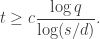
Theorem 12.1. [65] Let f:[q]^{d}\to [q]^{q} be d-wise uniform. Let q be a power of 2 and c\log q\le d\le q^{c}. Then any data structure with w=\log q using space s (which recall is measured in words of w bits) and time t has:

\begin{aligned} t\geq c\frac {\log q}{\log (s/d)}. \end{aligned}

Interpreting the input as coefficients of a degree d-1 univariate polynomial over \mathbb {F}_{q} and outputting its evaluations shows that such functions exists, and are in P. Below we give a surprising data structure that nearly matches the theorem.

To match previous parameters note that n=d\log q=dw, and m=\log q. Hence the bound is t\ge c(\log m)/\log (sw/n). Note that sw is the space of the data structure measured in bits. It follows that if sw is linear in n then t\ge c\log m. This result remains non-trivial for s slightly super-linear. But remarkably, if sw=n^{1+c} then nothing is known (for m power in n one only gets t\ge c).

ProofThe idea in the proof is to find a subset S of less than d memory cells that still allows us to answer \ge d queries. This is impossible, since we can’t generate d uniform outputs from less than d memory cells.

Let p:=1/q^{1/4t}. Include each memory bit in S with probability p, independently. By Theorem 2.7, \mathbb {P}[|S|\ge cps]\le 2^{-cps}.

We are still able to answer a query if all of its memory bits fall in S. The probability that this happens is p^{t}=1/q^{1/4}. We now claim that with probability \ge 1/q^{c}, we can still answer \sqrt {q} queries. Indeed, let B be the number of queries we cannot answer. We have \mathbb {E}[|B|]\le q(1-q^{1/4}). And so

\begin{aligned} \mathbb {P}[B\ge q(1-1/\sqrt {q})]\le \frac {1-q^{1/4}}{1-\sqrt {q}}\le 1-q^{c}. \end{aligned}

Thus, if the inequality 2^{-cps}\leq 1/q^{c} holds then there exists a set S of cps bits with which we can answer \ge \sqrt {q}>d queries. Hence we reach a contradiction if

\begin{aligned} c\log q\le cps<d. \end{aligned}="" Because d>c\log q by assumption, and increasing s only make the problem easier, we reach a contradiction if cps<d, and="" the="" result="" follows.="" QED

Next we show a conceptually simple data structure which nearly matches the lower bound. For simplicity we focus on data structures which use space q^{\epsilon } – recall in this case the previous result does not give anything. We will show this is for good reasons, there are data structures where the time is constant. We will only show c_{\epsilon }d-wise independence, as opposed to d-wise, but the proof techniques next and above generalize to other settings of parameters.

Theorem 12.2. There is a map f:[q]^{d}\to [q]^{q} which is c_{\epsilon }d-wise uniform and has a data structure with w=\log q space s=dq^{\epsilon } and time c_{\epsilon }, for any \epsilon and q which is a power of 2.

To give a sense of the parameters, let for example q=d^{10}.

ProofWe fill the memory with s evaluations of the input polynomial. Then we pick a random bipartite graph with s nodes on the left and q nodes on the right. Every node on the right side has degree g. We answer each query by summing the corresponding cells in s. Let d':=d/g. To show d'-wise uniformity it suffices to show that for any subset R\subseteq [q] on the right-hand side of size d', the sum of the corresponding memory cells is uniform in \mathbb {F}_{q}. For this in turn it suffices that R has a unique neighbor. And for that, finally, it suffices that R has a neighborhood of size greater than \frac {g|R|}{2} (because if every element in the neighborhood of R has two neighbors in R then R has a neighborhood of size less than g|r| 2).

Note here we are using that the neighborhood has size \le gd'=d, and so the memory is d-wise uniform.

We pick the graph at random and show that it has the latter property with non-zero probability.
[Standard calculations follow that wordpress has trouble displaying… wait for the book draft, I guess.]
QED

12.1.1 Succinct data structures

Succinct data structures are those where the space is close to the minimum, n. Specifically, we let s=n+r for some r=o(n) called redundancy. Unsurprisingly, stronger bounds can be probed in this setting. But, surprisingly, again these stronger bounds were shown to be tight. Moreover, it was shown that improving the bounds would imply stronger circuit lower bounds.

To illustrate, consider the ECC problem f:\{0,1\} ^{n}\to \{0,1\} ^{m} where f is an error-correcting code (with constant relative distance) and m is linear in n.

Theorem 12.3. [26] Any data-structure for the ECC problem with w=1 using space n+r requires time \ge cn/r.

This is nearly matched by the following result.

Theorem 12.4. [81] There is an ECC problem s.t. for any r it has a data structure with w=1, space n+r, and time c(n/r)\log ^{3}n.

Moreover, it was shown that proving a time lower bound of (n/r)\log ^{c}n would imply new circuit lower bounds. The latter result refers to bounds on the number of wires in circuits with arbitrary gates. But the following connection with the standard circuit model is also known.

Theorem 12.5. [81] Let f:\{0,1\} ^{n}\to \{0,1\} ^{am} be a function computable by bounded fan-in circuits with bm wires and depth b\log m, for constants a,b. Then f has a data structure with space n+o(n) and time n^{o(1)}.

Hence, proving n^{\epsilon } time lower bounds for succinct data structures would give functions that cannot be computed by linear-size log-depth circuits, cf. 9.3.

12.1.2 Succincter: The trits problem

In this section we present a cute and fundamental data-structure problem with a shocking and counterintuitive solution. The trits problem is to compute f:[3]^{n}\to (\{0,1\} ^{2})^{n} where on input n “trits” (i.e., ternary elements) (t_{1},t_{2},\ldots ,t_{n})\in [3]^{n} f outputs their representations using two bits per trit.

Example 12.1. For n=1, we have f(0)=00,f(1)=01,f(2)=10.

Note that the input ranges over 3^{n} elements, and so the minimum space of the data structure is s=\lceil \log _{2}3^{n}\rceil =\lceil n\log _{2}3\rceil \approx n\cdot 1.584\ldots This will be our benchmark for space. One can encode the input to f as before using bits without loss of generality, but the current choice simplifies the exposition.

Simple solutions:
  • The simplest solution (cf. 12.2) to this problem is to use 2 bits per t_{i}. With such an encoding we can retrieve each t_{i}\in [3] by reading just 2 bits (which is optimal). The space used is s=2n and we have linear redundancy.
  • Another solution (cf. again 12.2) to this problem is what is called arithmetic coding: we think of the concatenated elements as forming a ternary number between 0 and 3^{n}-1, and we write down its binary representation. To retrieve t_{i} it seems we need to read all the input bits, but the space needed is optimal.
  • For this and other problems, we can trade between these two extreme as follows. Group the t_{i}’s into blocks of t. Encode each block with arithmetic coding. The retrieval time will be ct bits and the needed space will be (n/t)\lceil t\log _{2}3\rceil \leq n\log _{2}3+n/t (assuming t divides n). This is block-wise arithmetic coding. It provides a power trade-off between retrieval time and redundancy. (Using number-theoretic results on logarithmic forms, one can show [80] that this last inequality is tight up to changing n/t into n/t^{c}.)

The shocking solution: An exponential (!) trade-off

We now present an exponential trade-off: retrieval time ct bits and redundancy n/2^{t}+c. In particular, if we set t=c\log n, we get retrieval time O(\log n) and redundancy O(1). Moreover, the bits read are all consecutive, so with word size w=\log n this can be implemented in constant time. To repeat, we can encode the trits with constant redundancy and retrieve each in constant time. This solution can also be made dynamic.

Theorem 12.6. [5321] The trits problem has a data structure with space n\log _{2}3+n/2^{t}+c (i.e., redundancy n/2^{t}+c) and time ct, for any t and with word size w=1. For word wise w=\log n the time is constant.

Next we present the proof.

Definition 12.3 (Encoding and redundancy). An encoding of a set A into a set B is a one-to-one (a.k.a. injective) map f:A\to B. The redundancy of the encoding f is \log _{2}|B|-\log _{2}|A|.

The following lemma gives the building-block encoding we will use.

Lemma 12.1. For all sets X and Y, there is an integer b, a set K and an encoding

\begin{aligned} f:\left (X\times Y\right )\rightarrow \left (\{0,1\} ^{b}\times K\right ) \end{aligned}

such that (1) f has redundancy \le c/\sqrt {|Y|}, and (2) x\in X can be recovered just by reading the b bits in f(x,y).

Note that (1) says that b+\log |K|-\log |X|-\log |Y|\le c/\sqrt {|Y|}. For (2) to hold we must have b\ge \log |X|. Combining this with the previous expression we obtain \log |K|-\log |Y|\le c/\sqrt {|Y|}. In particular we get that |K|\le 2^{c}\cdot |Y| (in fact it will be the case that |K|\le c\cdot \sqrt {|Y|}, but the looser bound is sufficient).

The basic idea for proving the lemma is to break Y into C\times K and then encode X\times C by using b bits:

\begin{aligned} X\times Y\rightarrow X\times C\times K\rightarrow \{0,1\} ^{b}\times K. \end{aligned}

There is however a subtle point. If we insist on always having |C| equal to, say, \sqrt {|Y|} or some other quantity, then one can cook up sets that make us waste a lot (i.e., almost one bit) of space. The same of course happens in the more basic approach that just sets Y=K and encodes all of X with b bits. The main idea will be to “reason backwards,” i.e., we will first pick b and then try to stuff as much as possible inside \{0,1\} ^{b}. Still, our choice of b will make |C| about \sqrt {|Y|}.

ProofPick any two sets X and Y, where |Y|>1 without loss of generality. Define b:=\left \lceil \log _{2}\left (|X|\cdot \sqrt {|Y|}\right )\right \rceil , and let B:=\{0,1\} ^{b}. To simplify notation, define d:=2^{b}/|X|. Note c\sqrt {|Y|}\le d\le c\sqrt {|Y|}.

How much can we stuff into B? For a set C of size |C|=\left \lfloor |B|/|X|\right \rfloor , we can encode elements from X\times C in B. The redundancy of such an encoding can be bounded as follows:

To calculate the total redundancy, we still need to examine the encoding from Y to C\times K. Choose K of size |K|=\left \lceil |Y|/|C|\right \rceil , so that this encoding is possible. With a calculation similar to the previous one, we see that the redundancy is:

The total redundancy is then c/\sqrt {|Y|}, which gives (1).

For (2), it is clear from the construction that any x\in X can be recovered from the element of B only. QED

Proof of Theorem 12.6 Break the ternary elements into blocks of size t: (t'_{1},t'_{2},\ldots ,t'_{n/t})\in T_{1}\times T_{2}\times \ldots \times T_{n/t}, where T_{i}=[3]^{t} for all i. The encoding, illustrated in Figure 1, is constructed as follows, where we use f_{L} to refer to the encoding guaranteed by Lemma Lemma 12.1.

Compute f_{L}(t'_{1},t'_{2})=(b_{1},k_{1})\in B_{1}\times K_{1}.

For i=2,\ldots ,n/t-1 compute f_{L}(k_{i-1},t'_{i+1}):=(b_{i},k_{i})\in B_{i}\times K_{i}.

Encode k_{n/t-1} in binary as b_{n/t} using arithmetic coding.

The final encoding is (b_{1},b_{2},\ldots ,b_{n/t}). We now compute the redundancy and retrieval time.

Redundancy: From (1) in Lemma 12.1, the first n/t-1 encodings have redundancy c3^{-t/2}\le 1/2^{ct}. For the last (arithmetic) encoding, the redundancy is at most 1. So the total redundancy is at most \displaystyle \left (\frac {n}{t}-1\right )\cdot \frac {1}{2^{ct}}+1=\frac {n}{2^{ct}}+c. One can visualize this as a “hybrid argument” transforming a product of blocks of ternary elements into a product of blocks of binary elements, one block at the time.

Retrieval Time: Say that we want to recover some t_{j} which is in block t'_{i}. To recover block t'_{i}, Lemma 12.1 guarantees that we only need to look at b_{i-1} and b_{i}. This is because k_{i-1} can be recovered by reading only b_{i}, and t'_{i} can be recovered by reading k_{i-1} and b_{i-1}. Thus to complete the proof it suffices to show that each b_{i} has length ct.

This is not completely obvious because one might have thought that the K_{i} become larger and larger, and so we apply the lemma to larger and larger inputs and the B_{i} get large too. However, recall that each |K_{i}|\le c|T_{i}|=c3^{t} from the comment after the statement of Lemma 12.1. Hence, every time we apply the lemma on an input of size at most s\le 3^{ct}. Since the lemma wastes little entropy (by (1) in Lemma 12.1), none of its outputs can be much larger than its input, and so |B_{i}|=2^{ct}.


PIC

Figure 12.1: Succinct Encoding


QED

12.2 Dynamic data structures

We now study dynamic data structures. As we mentioned, here the input is not fixed but can be modified by the queries.

Definition 12.4. Fix an error-correcting code \text {ECC}:\{0,1\} ^{n}\to \{0,1\} ^{m} where m\le cn and \Delta (\text {ECC}(x),\text {ECC}(y))\ge c for any x\ne y in \{0,1\} ^{n}. Here \Delta (u,v) is the relative distance, the fraction of bit positions where u and v differ.

The \text {ECC} problem asks to support operations, starting with the all-zero message:

M(i,b) for i\in \{1,2,\ldots ,n\} and b\in \{0,1\} which sets bit i of the message to b, and

C(i) for i\in \{1,2,\ldots ,m\} which returns bit i of the codeword corresponding to the current message.

The time of a dynamic data structure is the maximum number of read/write operations in memory cells required to support an operation.

Theorem 12.7. The \text {ECC} problem requires time t\ge c\log _{w}n\ge (c\log n)/\log \log n for cell size w:=\log n.

One might wonder if stronger bounds can be shown for this problem. But in fact there exist codes for which the bounds are nearly tight.

Theorem 12.8. [81]There exists codes for which the ECC problem can be solved in time c\log ^{2}n with cell size w=1.

The technique in the proof of Theorem 12.7 is from [24] and can be applied to many other natural problems, leading to tight results in several cases, see Exercise ??. It is not far from the state-of-the art in this area, which is \log ^{1+c}n [42].

Proof of Theorem 12.7 Pick x\in \{0,1\} ^{n} uniformly and i\in \{1,2,\ldots ,m\} uniformly, and consider the sequence of operations

\begin{aligned} M(1,x_{1}),M(2,x_{2}),\ldots ,M(n,x_{n}),C(i). \end{aligned}

That is, we set the message to a uniform x one bit at a time, and then ask for a uniformly selected bit of the codeword \text {ECC}(x), which we also denote by C_{x}=C_{x}(1),C_{x}(2),\ldots ,C_{x}(n).

We divide the n operations M(i,x_{i}) into consecutive blocks, called epochs. Epoch e consists of n/w^{3e} operations. Hence we can have at least E:=c\log _{w}n epochs, and we can assume that we have exactly this many epochs (by discarding some bits of n if necessary).

The geometrically decaying size of epochs is chosen so that the number of message bits set during an epoch e is much more than all the cells written by the data structure in future epochs.

A key idea of the proof is to see what happens when the cells written during a certain epoch are ignored, or reverted to their contents right before the epoch. Specifically, after the execution of the M operations, we can associate to each memory cell the last epoch during which this cell was written. Let D^{e}(x) denote the memory cells of the data structure after the first n operations M, but with the change that the cells that were written last during epoch e are replaced with their contents right before epoch e. Define C_{x}^{e}(i) to be the result of the data structure algorithm for C(i) on D^{e}(x), and C_{x}^{e}=C_{x}^{e}(1),C_{x}^{e}(2),\ldots ,C_{x}^{e}(n).

Let t(x,i,e) equal 1 if C(i), executed after the first n operations M, reads a cell that was last written in epoch e, and 0 otherwise. We have

\begin{aligned} t\ge \max _{x,i}\sum _{e}t(x,i,e)\ge \mathbb {E}_{x,i}\sum _{e}t(x,i,e)=\sum _{e}\mathbb {E}_{x,i}t(x,i,e)\ge \sum _{e}\mathbb {E}_{x}\Delta (C_{x},C_{x}^{e}),~~~~(12.1) \end{aligned}

where the last inequality holds because C_{x}^{e}(i)\ne C_{x}(i) implies t(x,i,e)\ge 1.

We now claim that if t\le w then \mathbb {E}_{x}\Delta (C_{x},C_{x}^{e})\ge c for every e. This concludes the proof.

In the remainder we justify the claim. Fix arbitrarily the bits of x set before Epoch e. For a uniform setting of the remaining bits of x, note that the message ranges over at least

\begin{aligned} 2^{n/w^{3e}} \end{aligned}

codewords. On the other hand, we claim that C_{x}^{e} ranges over much fewer strings. Indeed, the total number of cells written in all epochs after e is at most

\begin{aligned} t\sum _{i\ge e+1}n/w^{3i}\le ctn/w^{3(e+1)}. \end{aligned}

We can describe all these cells by writing down their indices and contents using B:=ctn/w^{3e+2} bits. Note that this information can depend on the operations performed during Epoch e, but the point is that it takes few possible values overall. Since the cells last changed during Epoch e are reverted to their contents before Epoch e, this information suffices to describe D^{e}(x), and hence C_{x}^{e}. Therefore, C_{x}^{e} ranges over \le 2^{B} strings.

For each string in the range of C_{x}^{e} at most two codewords can have relative distance \le c, for else you’d have two codewords at distance \le 2c, violating the distance of the code.

Hence except with probability 2\cdot 2^{B}/2^{n/w^{3e}} over x, we have \Delta (C_{x},C_{x}^{e})\ge c. If t_{M}\le w then the first probability is \le 0.1, and so \mathbb {E}_{x}\Delta (C_{x},C_{x}^{e})\ge c, proving the claim. QED

Exercise 12.4. Explain how to conclude the proof given the claim.

12.3 Notes

The exposition of the trits problem is from [76].

References

[1]   Amir Abboud, Arturs Backurs, and Virginia Vassilevska Williams. Tight hardness results for LCS and other sequence similarity measures. In Venkatesan Guruswami, editor, IEEE 56th Annual Symposium on Foundations of Computer Science, FOCS 2015, Berkeley, CA, USA, 17-20 October, 2015, pages 59–78. IEEE Computer Society, 2015.

[2]   Leonard Adleman. Two theorems on random polynomial time. In 19th IEEE Symp. on Foundations of Computer Science (FOCS), pages 75–83. 1978.

[3]   Mikl�s Ajtai. \Sigma \sp {1}\sb {1}-formulae on finite structures. Annals of Pure and Applied Logic, 24(1):1–48, 1983.

[4]   Mikl�s Ajtai. A non-linear time lower bound for boolean branching programs. Theory of Computing, 1(1):149–176, 2005.

[5]   Eric Allender. A note on the power of threshold circuits. In 30th Symposium on Foundations of Computer Science, pages 580–584, Research Triangle Park, North Carolina, 30 October–1 November 1989. IEEE.

[6]   Eric Allender. The division breakthroughs. Bulletin of the EATCS, 74:61–77, 2001.

[7]   Eric Allender and Michal Koucký. Amplifying lower bounds by means of self-reducibility. J. of the ACM, 57(3), 2010.

[8]   Noga Alon, Oded Goldreich, Johan H�stad, and Ren� Peralta. Simple constructions of almost k-wise independent random variables. Random Structures & Algorithms, 3(3):289–304, 1992.

[9]   Dana Angluin and Leslie G. Valiant. Fast probabilistic algorithms for hamiltonian circuits and matchings. J. Comput. Syst. Sci., 18(2):155–193, 1979.

[10]   Sanjeev Arora, Carsten Lund, Rajeev Motwani, Madhu Sudan, and Mario Szegedy. Proof verification and the hardness of approximation problems. J. of the ACM, 45(3):501–555, May 1998.

[11]   Arturs Backurs and Piotr Indyk. Edit distance cannot be computed in strongly subquadratic time (unless SETH is false). SIAM J. Comput., 47(3):1087–1097, 2018.

[12]   Kenneth E. Batcher. Sorting networks and their applications. In AFIPS Spring Joint Computing Conference, volume 32, pages 307–314, 1968.

[13]   Paul Beame, Stephen A. Cook, and H. James Hoover. Log depth circuits for division and related problems. SIAM J. Comput., 15(4):994–1003, 1986.

[14]   Paul Beame, Michael Saks, Xiaodong Sun, and Erik Vee. Time-space trade-off lower bounds for randomized computation of decision problems. J. of the ACM, 50(2):154–195, 2003.

[15]   Michael Ben-Or and Richard Cleve. Computing algebraic formulas using a constant number of registers. SIAM J. on Computing, 21(1):54–58, 1992.

[16]   Samuel R. Buss and Ryan Williams. Limits on alternation trading proofs for time-space lower bounds. Comput. Complex., 24(3):533–600, 2015.

[17]   Lijie Chen and Roei Tell. Bootstrapping results for threshold circuits “just beyond” known lower bounds. In Moses Charikar and Edith Cohen, editors, Proceedings of the 51st Annual ACM SIGACT Symposium on Theory of Computing, STOC 2019, Phoenix, AZ, USA, June 23-26, 2019, pages 34–41. ACM, 2019.

[18]   Richard Cleve. Towards optimal simulations of formulas by bounded-width programs. Computational Complexity, 1:91–105, 1991.

[19]   Stephen A. Cook. A hierarchy for nondeterministic time complexity. J. of Computer and System Sciences, 7(4):343–353, 1973.

[20]   L. Csanky. Fast parallel matrix inversion algorithms. SIAM J. Comput., 5(4):618–623, 1976.

[21]   Yevgeniy Dodis, Mihai Pǎtraşcu, and Mikkel Thorup. Changing base without losing space. In 42nd ACM Symp. on the Theory of Computing (STOC), pages 593–602. ACM, 2010.

[22]   Lance Fortnow. Time-space tradeoffs for satisfiability. J. Comput. Syst. Sci., 60(2):337–353, 2000.

[23]   Aviezri S. Fraenkel and David Lichtenstein. Computing a perfect strategy for n x n chess requires time exponential in n. J. Comb. Theory, Ser. A, 31(2):199–214, 1981.

[24]   Michael L. Fredman and Michael E. Saks. The cell probe complexity of dynamic data structures. In ACM Symp. on the Theory of Computing (STOC), pages 345–354, 1989.

[25]   Anka Gajentaan and Mark H. Overmars. On a class of {O}(n^2) problems in computational geometry. Comput. Geom., 5:165–185, 1995.

[26]   Anna G�l and Peter Bro Miltersen. The cell probe complexity of succinct data structures. Theoretical Computer Science, 379(3):405–417, 2007.

[27]   M. R. Garey and David S. Johnson. Computers and Intractability: A Guide to the Theory of NP-Completeness. W. H. Freeman, 1979.

[28]   K. G�del. �ber formal unentscheidbare s�tze der Principia Mathematica und verwandter systeme I. Monatsh. Math. Phys., 38, 1931.

[29]   Oded Goldreich. Computational Complexity: A Conceptual Perspective. Cambridge University Press, 2008.

[30]   Raymond Greenlaw, H. James Hoover, and Walter Ruzzo. Limits to Parallel Computation: P-Completeness Theory. 02 2001.

[31]   David Harvey and Joris van der Hoeven. Integer multiplication in time O(n\mathrm {log}\, n). Annals of Mathematics, 193(2):563 – 617, 2021.

[32]   F. C. Hennie. One-tape, off-line turing machine computations. Information and Control, 8(6):553–578, 1965.

[33]   Fred Hennie and Richard Stearns. Two-tape simulation of multitape turing machines. J. of the ACM, 13:533–546, October 1966.

[34]   John E. Hopcroft, Wolfgang J. Paul, and Leslie G. Valiant. On time versus space. J. ACM, 24(2):332–337, 1977.

[35]   Russell Impagliazzo and Ramamohan Paturi. The complexity of k-sat. In IEEE Conf. on Computational Complexity (CCC), pages 237–, 1999.

[36]   Russell Impagliazzo, Ramamohan Paturi, and Michael E. Saks. Size-depth tradeoffs for threshold circuits. SIAM J. Comput., 26(3):693–707, 1997.

[37]   Russell Impagliazzo, Ramamohan Paturi, and Francis Zane. Which problems have strongly exponential complexity? J. Computer & Systems Sciences, 63(4):512–530, Dec 2001.

[38]   Russell Impagliazzo and Avi Wigderson. \mathit {P} = \mathit {BPP} if E requires exponential circuits: Derandomizing the XOR lemma. In 29th ACM Symp. on the Theory of Computing (STOC), pages 220–229. ACM, 1997.

[39]   Richard M. Karp and Richard J. Lipton. Turing machines that take advice. L’Enseignement Math�matique. Revue Internationale. IIe S�rie, 28(3-4):191–209, 1982.

[40]   Kojiro Kobayashi. On the structure of one-tape nondeterministic turing machine time hierarchy. Theor. Comput. Sci., 40:175–193, 1985.

[41]   Swastik Kopparty and Srikanth Srinivasan. Certifying polynomials for AC\({}^{\mbox {0}}\)[\(\oplus \)] circuits, with applications to lower bounds and circuit compression. Theory of Computing, 14(1):1–24, 2018.

[42]   Kasper Green Larsen, Omri Weinstein, and Huacheng Yu. Crossing the logarithmic barrier for dynamic boolean data structure lower bounds. SIAM J. Comput., 49(5), 2020.

[43]   Leonid A. Levin. Universal sequential search problems. Problemy Peredachi Informatsii, 9(3):115–116, 1973.

[44]   Carsten Lund, Lance Fortnow, Howard Karloff, and Noam Nisan. Algebraic methods for interactive proof systems. J. of the ACM, 39(4):859–868, October 1992.

[45]   O. B. Lupanov. A method of circuit synthesis. Izv. VUZ Radiofiz., 1:120–140, 1958.

[46]   Wolfgang Maass and Amir Schorr. Speed-up of Turing machines with one work tape and a two-way input tape. SIAM J. on Computing, 16(1):195–202, 1987.

[47]   David A. Mix Barrington. Bounded-width polynomial-size branching programs recognize exactly those languages in NC1. J. of Computer and System Sciences, 38(1):150–164, 1989.

[48]   Joseph Naor and Moni Naor. Small-bias probability spaces: efficient constructions and applications. SIAM J. on Computing, 22(4):838–856, 1993.

[49]   E. I. Nechiporuk. A boolean function. Soviet Mathematics-Doklady, 169(4):765–766, 1966.

[50]   Valery A. Nepomnjaščiĭ. Rudimentary predicates and Turing calculations. Soviet Mathematics-Doklady, 11(6):1462–1465, 1970.

[51]   NEU. From RAM to SAT. Available at http://www.ccs.neu.edu/home/viola/, 2012.

[52]   Christos H. Papadimitriou and Mihalis Yannakakis. Optimization, approximation, and complexity classes. J. Comput. Syst. Sci., 43(3):425–440, 1991.

[53]   Mihai Pǎtraşcu. Succincter. In 49th IEEE Symp. on Foundations of Computer Science (FOCS). IEEE, 2008.

[54]   Wolfgang J. Paul, Nicholas Pippenger, Endre Szemer�di, and William T. Trotter. On determinism versus non-determinism and related problems (preliminary version). In IEEE Symp. on Foundations of Computer Science (FOCS), pages 429–438, 1983.

[55]   Nicholas Pippenger and Michael J. Fischer. Relations among complexity measures. J. of the ACM, 26(2):361–381, 1979.

[56]   Alexander Razborov. Lower bounds on the dimension of schemes of bounded depth in a complete basis containing the logical addition function. Akademiya Nauk SSSR. Matematicheskie Zametki, 41(4):598–607, 1987. English translation in Mathematical Notes of the Academy of Sci. of the USSR, 41(4):333-338, 1987.

[57]   Omer Reingold. Undirected connectivity in log-space. J. of the ACM, 55(4), 2008.

[58]   J. M. Robson. N by N checkers is exptime complete. SIAM J. Comput., 13(2):252–267, 1984.

[59]   Rahul Santhanam. On separators, segregators and time versus space. In IEEE Conf. on Computational Complexity (CCC), pages 286–294, 2001.

[60]   Walter J. Savitch. Relationships between nondeterministic and deterministic tape complexities. Journal of Computer and System Sciences, 4(2):177–192, 1970.

[61]   Arnold Sch�nhage. Storage modification machines. SIAM J. Comput., 9(3):490–508, 1980.

[62]   Adi Shamir. IP = PSPACE. J. of the ACM, 39(4):869–877, October 1992.

[63]   Claude E. Shannon. The synthesis of two-terminal switching circuits. Bell System Tech. J., 28:59–98, 1949.

[64]   Victor Shoup. New algorithms for finding irreducible polynomials over finite fields. Mathematics of Computation, 54(189):435–447, 1990.

[65]   Alan Siegel. On universal classes of extremely random constant-time hash functions. SIAM J. on Computing, 33(3):505–543, 2004.

[66]   Michael Sipser. A complexity theoretic approach to randomness. In ACM Symp. on the Theory of Computing (STOC), pages 330–335, 1983.

[67]   Roman Smolensky. Algebraic methods in the theory of lower bounds for Boolean circuit complexity. In 19th ACM Symp. on the Theory of Computing (STOC), pages 77–82. ACM, 1987.

[68]   Larry Stockmeyer and Albert R. Meyer. Cosmological lower bound on the circuit complexity of a small problem in logic. J. ACM, 49(6):753–784, 2002.

[69]   Seinosuke Toda. PP is as hard as the polynomial-time hierarchy. SIAM J. on Computing, 20(5):865–877, 1991.

[70]   Alan M. Turing. On computable numbers, with an application to the entscheidungsproblem. Proc. London Math. Soc., s2-42(1):230–265, 1937.

[71]   Leslie G. Valiant. Graph-theoretic arguments in low-level complexity. In 6th Symposium on Mathematical Foundations of Computer Science, volume 53 of Lecture Notes in Computer Science, pages 162–176. Springer, 1977.

[72]   Leslie G. Valiant and Vijay V. Vazirani. NP is as easy as detecting unique solutions. Theor. Comput. Sci., 47(3):85–93, 1986.

[73]   Dieter van Melkebeek. A survey of lower bounds for satisfiability and related problems. Foundations and Trends in Theoretical Computer Science, 2(3):197–303, 2006.

[74]   Dieter van Melkebeek and Ran Raz. A time lower bound for satisfiability. Theor. Comput. Sci., 348(2-3):311–320, 2005.

[75]   N. V. Vinodchandran. A note on the circuit complexity of PP. Theor. Comput. Sci., 347(1-2):415–418, 2005.

[76]   Emanuele Viola. Gems of theoretical computer science. Lecture notes of the class taught at Northeastern University. Available at http://www.ccs.neu.edu/home/viola/classes/gems-08/index.html, 2009.

[77]   Emanuele Viola. On approximate majority and probabilistic time. Computational Complexity, 18(3):337–375, 2009.

[78]   Emanuele Viola. On the power of small-depth computation. Foundations and Trends in Theoretical Computer Science, 5(1):1–72, 2009.

[79]   Emanuele Viola. Reducing 3XOR to listing triangles, an exposition. Available at http://www.ccs.neu.edu/home/viola/, 2011.

[80]   Emanuele Viola. Bit-probe lower bounds for succinct data structures. SIAM J. on Computing, 41(6):1593–1604, 2012.

[81]   Emanuele Viola. Lower bounds for data structures with space close to maximum imply circuit lower bounds. Theory of Computing, 15:1–9, 2019. Available at http://www.ccs.neu.edu/home/viola/.

[82]   Emanuele Viola. Pseudorandom bits and lower bounds for randomized turing machines. Theory of Computing, 18(10):1–12, 2022.

Mathematics of the impossible, Chapter 11, Proofs

The notion of proof is pervasive. We have seen many proofs in this book until now. But the notion extends to others realms of knowledge, including empirical science, law, and more. Complexity theory has contributed a great deal to the notion of proof, with important applications in several areas such as cryptography.

11.1 Static proofs

As remarked in section 5.1.0.1, we can think of problems in \text {NP} as those admitting a solution that can be verified efficiently, namely in \text {P}. Let us repeat the definition of \text {NP} using the suggestive letter V for verifier.

Definition 11.1. A function f:X\subseteq \{0,1\}^* \to \{0,1\} is in \text {NP} iff there is V\in \text {P} (called “verifier”) and d\in \mathbb {N} s.t.:

\begin{aligned} f(x)=1\Leftrightarrow \exists y\in \{0,1\} ^{|x|^{d}}:V(x,y)=1. \end{aligned}

We are naturally interested in fast proof verification, and especially the complexity of V. It turns out that proofs can be encoded in a format that allows for very efficient verification. This message is already in the following.

Theorem 11.1. For any input length n, V in Definition 11.1 can be taken to be a 3CNF of size n^{d}.

That is, whereas when defining \text {NP} as a proof system we considered arbitrary verifiers V in P, in fact the definition is unchanged if one selects a very restricted class of verifiers: small 3CNFs.

ProofThis is just a restatement of Theorem 5.1. QED

This extreme reduction in the verifier’s complexity is possible because we are allowing proofs to be long, longer than the original verifier’s running time. If we don’t allow for that, such a reduction is not known. Such “bounded proofs” are very interesting to study, but we shall not do so now.

Instead, we ask for more. The 3CNF in the above theorem still depends on the entire proof. We can ask for a verifier that only depends on few bits of the proof. Taking this to the extreme, we can ask whether V can only read a constant number of bits from y. Without randomness, this is impossible.

Exercise 11.1. Suppose V in Definition 11.1 only reads \le d bits of y, for a constant d. Show that the corresponding class would be the same as P.

Surprisingly, if we allow randomness this is possible. Moreover, the use of randomness is fairly limited – only logarithmically many bits – yielding the following central characterization.

Theorem 11.2. A function f:X\subseteq \{0,1\}^* \to \{0,1\} is in \text {NP} iff there is V\in \text {P} and d\in \mathbb {N} s.t.:

f(x)=1\Rightarrow \exists y\in \{0,1\} ^{|x|^{d}}:\mathbb {P}_{r\in \{0,1\} ^{d\log |x|}}[V(x,y,r)=1]=1,

f(x)=0\Rightarrow \forall y\in \{0,1\} ^{|x|^{d}}:\mathbb {P}_{r\in \{0,1\} ^{d\log |x|}}[V(x,y,r)=1]<0.01,

and moreover V reads \le d bits of y.

Exercise 11.2. Prove the “only if” in Theorem 11.2 in the specific case f=0.01\text {-Gap-3Sat}.

Given this exercise, the “only if” direction for any problem in NP follows from the advanced result that any problem in NP can be map reduced to 0.01-Gap-3Sat (which is essentially Theorem 4.7, except we did not claim map reductions or a specific constant there).

Exercise 11.3. Prove the “if” in Theorem 11.2.

11.2 Zero-knowledge

In Theorem 11.2 the verifier gains “constant confidence” about the validity of the proof, just be inspecting a constant number of bits. Hence the verifier “learns” at most a constant number of bits of the proof. This is remarkable, but we can further ask if we can modify the proof so that the verifier “learns nothing” about the proof. Such proofs are called zero knowledge and are extensively studied and applied.

We sketch how this is done for Gap-3Color, which is also NP-complete. Rather than a single proof y, now the verifier will receive a random proof Y. This Y is obtained from a 3 coloring y by randomly permuting colors (so for any y the corresponding Y is uniform over 6 colorings). The verifier will pick a random edge and inspect the corresponding endpoints, and accept if they are different.

The verifier learn nothing because all that they see is two random different color. One can formalize “learning nothing” by noting that the verifier can produce this distribution by themselves, without looking at the proof. (So why does the verifier gain anything from y? The fact that a proof y has been written down means that colors have been picked so that every two endpoints are uniform colors, something that the verifier is not easily able to reproduce.)

This gives a zero-knowledge proof for verifiers that follow the protocol of just inspecting an edge. In a cryptographic setting one has to worry about verifiers which don’t follow the protocol. Using cryptographic assumptions, one can force the verifiers to follow the protocol by considering an interactive proof: First a proof y is committed to but not revealed, then the verifier selects an edge to inspect, and only then the corresponding colors are revealed, and only those. This protocol lends itself to a physical implementation.

11.3 Interactive proofs

We now consider interactive proofs. Here the verifier V engages in a protocol with a prover P. Given an input x to both V and P, the verifier asks questions, the prover replies, the verifier asks more questions, and so on. The case of NP corresponds to the prover simply sending y to V.

It turns out that it suffices for the verifier to send uniformly random strings Q_{1},Q_{2},\ldots bits to P. This leads to a simple definition.

Definition 11.2. A function f:X\subseteq \{0,1\}^* \to \{0,1\} admits an efficient interactive proof, abbreviated IP, if there is V\in \text {P} and d\in \mathbb {N} such that for every x\in \{0,1\} ^{n}, letting b:=n^{d}:

  • If f(x)=1 then \exists P:\{0,1\}^* \to \{0,1\} ^{b} such that
    \begin{aligned} V\left (P(Q_{1}),P(Q_{1},Q_{2}),\ldots ,P(Q_{1},Q_{2},\ldots ,Q_{b})\right )=1 \end{aligned}

    for every Q_{1},Q_{2},\ldots ,Q_{b}\in \{0,1\} ^{b}.

  • If f(x)=0 then \forall P:\{0,1\}^* \to \{0,1\} ^{b} we have
    \begin{aligned} \mathbb {P}_{Q_{1},Q_{2},\ldots ,Q_{b}\in \{0,1\} ^{b}}\left [V\left (P(Q_{1}),P(Q_{1},Q_{2}),\ldots ,P(Q_{1},Q_{2},\ldots ,Q_{b})\right )=1\right ]\le 1/3. \end{aligned}

The following amazing result shows the power of interactive proofs, compared to non-interactive proofs. We can think of NP as “reading a book” and IP as “going to class and asking questions.” We don’t yet know how to replace teachers with books.

Theorem 11.3. [4158]\text { IP}=\text {PSpace}.

In the rest of this section we present the main ideas in the proof of 11.3, establishing a weaker result. In particular we show that IP contains problems not known to be in NP.

Theorem 11.4. Given a field \mathbb {F}, an arithmetic circuit C(x_{1},x_{2},\ldots ,x_{v}) over \mathbb {F} computing a polynomial of degree d, and an element s\in \mathbb {F}, deciding if

\begin{aligned} \sum _{x_{1},x_{2},\ldots ,x_{v}\in \{0,1\} }C(x_{1},x_{2},\ldots ,x_{v})=s~~~~(11.1) \end{aligned}

is in IP, whenever (1-d/q)^{v}\ge 2/3.

ProofIf v=1 then V can decide this question by itself, by evaluating the circuit. For larger v we give a way to reduce v by 1.

As the first prover answer, V expects a polynomial p of degree d in the variable x, which is meant to be

\begin{aligned} s'(x):=\sum _{x_{2},x_{3},\ldots ,x_{n}\in \{0,1\} }C(x,x_{2},x_{3}\ldots ,x_{n}). \end{aligned}

V checks if p(0)+p(1)=s, and if not rejects. Otherwise, it recursively runs the protocol to verify that

\begin{aligned} \sum _{x_{2},x_{3},\ldots ,x_{n}\in \{0,1\} }C(Q_{1},x_{2},x_{3},\ldots ,x_{n})=p(Q_{1}).~~~~(11.2) \end{aligned}

This concludes the description of the protocol. We now verify its correctness.

In case equation (??) is true, P can send polynomials that cause V to accept.

In case equation (??) is false, s'(0)+s'(1)\ne s. Hence, unless V rejects right away because p(0)+p(1)\ne s, we have p\ne s'. The polynomials p and s' have degree \le d. Hence by Lemma 2.3

\begin{aligned} \mathbb {P}_{Q_{1}}[p(Q_{1})\ne s'(Q_{1})]\ge 1-d/q. \end{aligned}

When this event occurs, equation (??) is again false, and we can repeat the argument. Overall, the probability that we maintain a false statement throughout the protocol is \ge (1-d/q)^{v}. QED

Corollary 11.1. Given a 3CNF formula \phi and k\in \mathbb {N}, deciding if \phi has exactly k satisfying assignments is in \text {IP}.

The proof uses a far-reaching technique: arithmetization. We construct an arithmetic circuit C_{\phi } over a field \mathbb {F} which agrees with \phi on boolean inputs, but that can then be evaluated over other elements of the field.

Exercise 11.4. Prove Corollary 11.1.

The study of interactive proofs is rich. Many aspects are of interest, including:

  • The efficiency of the prover (does it have to be unbounded, randomized, etc.), and of the verifier.
  • The number of rounds.
  • The tradeoff betwen the error and the other parameters.

References

[1]   Amir Abboud, Arturs Backurs, and Virginia Vassilevska Williams. Tight hardness results for LCS and other sequence similarity measures. In Venkatesan Guruswami, editor, IEEE 56th Annual Symposium on Foundations of Computer Science, FOCS 2015, Berkeley, CA, USA, 17-20 October, 2015, pages 59–78. IEEE Computer Society, 2015.

[2]   Leonard Adleman. Two theorems on random polynomial time. In 19th IEEE Symp. on Foundations of Computer Science (FOCS), pages 75–83. 1978.

[3]   Mikl�s Ajtai. \Sigma \sp {1}\sb {1}-formulae on finite structures. Annals of Pure and Applied Logic, 24(1):1–48, 1983.

[4]   Mikl�s Ajtai. A non-linear time lower bound for boolean branching programs. Theory of Computing, 1(1):149–176, 2005.

[5]   Eric Allender. A note on the power of threshold circuits. In 30th Symposium on Foundations of Computer Science, pages 580–584, Research Triangle Park, North Carolina, 30 October–1 November 1989. IEEE.

[6]   Eric Allender. The division breakthroughs. Bulletin of the EATCS, 74:61–77, 2001.

[7]   Eric Allender and Michal Koucký. Amplifying lower bounds by means of self-reducibility. J. of the ACM, 57(3), 2010.

[8]   Noga Alon, Oded Goldreich, Johan H�stad, and Ren� Peralta. Simple constructions of almost k-wise independent random variables. Random Structures & Algorithms, 3(3):289–304, 1992.

[9]   Dana Angluin and Leslie G. Valiant. Fast probabilistic algorithms for hamiltonian circuits and matchings. J. Comput. Syst. Sci., 18(2):155–193, 1979.

[10]   Sanjeev Arora, Carsten Lund, Rajeev Motwani, Madhu Sudan, and Mario Szegedy. Proof verification and the hardness of approximation problems. J. of the ACM, 45(3):501–555, May 1998.

[11]   Arturs Backurs and Piotr Indyk. Edit distance cannot be computed in strongly subquadratic time (unless SETH is false). SIAM J. Comput., 47(3):1087–1097, 2018.

[12]   Kenneth E. Batcher. Sorting networks and their applications. In AFIPS Spring Joint Computing Conference, volume 32, pages 307–314, 1968.

[13]   Paul Beame, Stephen A. Cook, and H. James Hoover. Log depth circuits for division and related problems. SIAM J. Comput., 15(4):994–1003, 1986.

[14]   Paul Beame, Michael Saks, Xiaodong Sun, and Erik Vee. Time-space trade-off lower bounds for randomized computation of decision problems. J. of the ACM, 50(2):154–195, 2003.

[15]   Michael Ben-Or and Richard Cleve. Computing algebraic formulas using a constant number of registers. SIAM J. on Computing, 21(1):54–58, 1992.

[16]   Samuel R. Buss and Ryan Williams. Limits on alternation trading proofs for time-space lower bounds. Comput. Complex., 24(3):533–600, 2015.

[17]   Lijie Chen and Roei Tell. Bootstrapping results for threshold circuits “just beyond” known lower bounds. In Moses Charikar and Edith Cohen, editors, Proceedings of the 51st Annual ACM SIGACT Symposium on Theory of Computing, STOC 2019, Phoenix, AZ, USA, June 23-26, 2019, pages 34–41. ACM, 2019.

[18]   Richard Cleve. Towards optimal simulations of formulas by bounded-width programs. Computational Complexity, 1:91–105, 1991.

[19]   Stephen A. Cook. A hierarchy for nondeterministic time complexity. J. of Computer and System Sciences, 7(4):343–353, 1973.

[20]   L. Csanky. Fast parallel matrix inversion algorithms. SIAM J. Comput., 5(4):618–623, 1976.

[21]   Lance Fortnow. Time-space tradeoffs for satisfiability. J. Comput. Syst. Sci., 60(2):337–353, 2000.

[22]   Aviezri S. Fraenkel and David Lichtenstein. Computing a perfect strategy for n x n chess requires time exponential in n. J. Comb. Theory, Ser. A, 31(2):199–214, 1981.

[23]   Michael L. Fredman and Michael E. Saks. The cell probe complexity of dynamic data structures. In ACM Symp. on the Theory of Computing (STOC), pages 345–354, 1989.

[24]   Anka Gajentaan and Mark H. Overmars. On a class of {O}(n^2) problems in computational geometry. Comput. Geom., 5:165–185, 1995.

[25]   M. R. Garey and David S. Johnson. Computers and Intractability: A Guide to the Theory of NP-Completeness. W. H. Freeman, 1979.

[26]   K. G�del. �ber formal unentscheidbare s�tze der Principia Mathematica und verwandter systeme I. Monatsh. Math. Phys., 38, 1931.

[27]   Oded Goldreich. Computational Complexity: A Conceptual Perspective. Cambridge University Press, 2008.

[28]   Raymond Greenlaw, H. James Hoover, and Walter Ruzzo. Limits to Parallel Computation: P-Completeness Theory. 02 2001.

[29]   David Harvey and Joris van der Hoeven. Integer multiplication in time O(n\mathrm {log}\, n). Annals of Mathematics, 193(2):563 – 617, 2021.

[30]   F. C. Hennie. One-tape, off-line turing machine computations. Information and Control, 8(6):553–578, 1965.

[31]   Fred Hennie and Richard Stearns. Two-tape simulation of multitape turing machines. J. of the ACM, 13:533–546, October 1966.

[32]   John E. Hopcroft, Wolfgang J. Paul, and Leslie G. Valiant. On time versus space. J. ACM, 24(2):332–337, 1977.

[33]   Russell Impagliazzo and Ramamohan Paturi. The complexity of k-sat. In IEEE Conf. on Computational Complexity (CCC), pages 237–, 1999.

[34]   Russell Impagliazzo, Ramamohan Paturi, and Michael E. Saks. Size-depth tradeoffs for threshold circuits. SIAM J. Comput., 26(3):693–707, 1997.

[35]   Russell Impagliazzo, Ramamohan Paturi, and Francis Zane. Which problems have strongly exponential complexity? J. Computer & Systems Sciences, 63(4):512–530, Dec 2001.

[36]   Russell Impagliazzo and Avi Wigderson. \mathit {P} = \mathit {BPP} if E requires exponential circuits: Derandomizing the XOR lemma. In 29th ACM Symp. on the Theory of Computing (STOC), pages 220–229. ACM, 1997.

[37]   Richard M. Karp and Richard J. Lipton. Turing machines that take advice. L’Enseignement Math�matique. Revue Internationale. IIe S�rie, 28(3-4):191–209, 1982.

[38]   Kojiro Kobayashi. On the structure of one-tape nondeterministic turing machine time hierarchy. Theor. Comput. Sci., 40:175–193, 1985.

[39]   Kasper Green Larsen, Omri Weinstein, and Huacheng Yu. Crossing the logarithmic barrier for dynamic boolean data structure lower bounds. SIAM J. Comput., 49(5), 2020.

[40]   Leonid A. Levin. Universal sequential search problems. Problemy Peredachi Informatsii, 9(3):115–116, 1973.

[41]   Carsten Lund, Lance Fortnow, Howard Karloff, and Noam Nisan. Algebraic methods for interactive proof systems. J. of the ACM, 39(4):859–868, October 1992.

[42]   O. B. Lupanov. A method of circuit synthesis. Izv. VUZ Radiofiz., 1:120–140, 1958.

[43]   Wolfgang Maass and Amir Schorr. Speed-up of Turing machines with one work tape and a two-way input tape. SIAM J. on Computing, 16(1):195–202, 1987.

[44]   David A. Mix Barrington. Bounded-width polynomial-size branching programs recognize exactly those languages in NC^1. J. of Computer and System Sciences, 38(1):150–164, 1989.

[45]   Joseph Naor and Moni Naor. Small-bias probability spaces: efficient constructions and applications. SIAM J. on Computing, 22(4):838–856, 1993.

[46]   E. I. Nechiporuk. A boolean function. Soviet Mathematics-Doklady, 169(4):765–766, 1966.

[47]   Valery A. Nepomnjaščiĭ. Rudimentary predicates and Turing calculations. Soviet Mathematics-Doklady, 11(6):1462–1465, 1970.

[48]   NEU. From RAM to SAT. Available at http://www.ccs.neu.edu/home/viola/, 2012.

[49]   Christos H. Papadimitriou and Mihalis Yannakakis. Optimization, approximation, and complexity classes. J. Comput. Syst. Sci., 43(3):425–440, 1991.

[50]   Wolfgang J. Paul, Nicholas Pippenger, Endre Szemer�di, and William T. Trotter. On determinism versus non-determinism and related problems (preliminary version). In IEEE Symp. on Foundations of Computer Science (FOCS), pages 429–438, 1983.

[51]   Nicholas Pippenger and Michael J. Fischer. Relations among complexity measures. J. of the ACM, 26(2):361–381, 1979.

[52]   Alexander Razborov. Lower bounds on the dimension of schemes of bounded depth in a complete basis containing the logical addition function. Akademiya Nauk SSSR. Matematicheskie Zametki, 41(4):598–607, 1987. English translation in Mathematical Notes of the Academy of Sci. of the USSR, 41(4):333-338, 1987.

[53]   Omer Reingold. Undirected connectivity in log-space. J. of the ACM, 55(4), 2008.

[54]   J. M. Robson. N by N checkers is exptime complete. SIAM J. Comput., 13(2):252–267, 1984.

[55]   Rahul Santhanam. On separators, segregators and time versus space. In IEEE Conf. on Computational Complexity (CCC), pages 286–294, 2001.

[56]   Walter J. Savitch. Relationships between nondeterministic and deterministic tape complexities. Journal of Computer and System Sciences, 4(2):177–192, 1970.

[57]   Arnold Sch�nhage. Storage modification machines. SIAM J. Comput., 9(3):490–508, 1980.

[58]   Adi Shamir. IP = PSPACE. J. of the ACM, 39(4):869–877, October 1992.

[59]   Claude E. Shannon. The synthesis of two-terminal switching circuits. Bell System Tech. J., 28:59–98, 1949.

[60]   Victor Shoup. New algorithms for finding irreducible polynomials over finite fields. Mathematics of Computation, 54(189):435–447, 1990.

[61]   Alan Siegel. On universal classes of extremely random constant-time hash functions. SIAM J. on Computing, 33(3):505–543, 2004.

[62]   Michael Sipser. A complexity theoretic approach to randomness. In ACM Symp. on the Theory of Computing (STOC), pages 330–335, 1983.

[63]   Roman Smolensky. Algebraic methods in the theory of lower bounds for Boolean circuit complexity. In 19th ACM Symp. on the Theory of Computing (STOC), pages 77–82. ACM, 1987.

[64]   Larry Stockmeyer and Albert R. Meyer. Cosmological lower bound on the circuit complexity of a small problem in logic. J. ACM, 49(6):753–784, 2002.

[65]   Seinosuke Toda. PP is as hard as the polynomial-time hierarchy. SIAM J. on Computing, 20(5):865–877, 1991.

[66]   Alan M. Turing. On computable numbers, with an application to the entscheidungsproblem. Proc. London Math. Soc., s2-42(1):230–265, 1937.

[67]   Leslie G. Valiant. Graph-theoretic arguments in low-level complexity. In 6th Symposium on Mathematical Foundations of Computer Science, volume 53 of Lecture Notes in Computer Science, pages 162–176. Springer, 1977.

[68]   Leslie G. Valiant and Vijay V. Vazirani. NP is as easy as detecting unique solutions. Theor. Comput. Sci., 47(3):85–93, 1986.

[69]   Dieter van Melkebeek. A survey of lower bounds for satisfiability and related problems. Foundations and Trends in Theoretical Computer Science, 2(3):197–303, 2006.

[70]   Dieter van Melkebeek and Ran Raz. A time lower bound for satisfiability. Theor. Comput. Sci., 348(2-3):311–320, 2005.

[71]   N. V. Vinodchandran. A note on the circuit complexity of PP. Theor. Comput. Sci., 347(1-2):415–418, 2005.

[72]   Emanuele Viola. On approximate majority and probabilistic time. Computational Complexity, 18(3):337–375, 2009.

[73]   Emanuele Viola. On the power of small-depth computation. Foundations and Trends in Theoretical Computer Science, 5(1):1–72, 2009.

[74]   Emanuele Viola. Reducing 3XOR to listing triangles, an exposition. Available at http://www.ccs.neu.edu/home/viola/, 2011.

[75]   Emanuele Viola. Lower bounds for data structures with space close to maximum imply circuit lower bounds. Theory of Computing, 15:1–9, 2019. Available at http://www.ccs.neu.edu/home/viola/.

[76]   Emanuele Viola. Pseudorandom bits and lower bounds for randomized turing machines. Theory of Computing, 18(10):1–12, 2022.

Mathematics of the impossible, Chapter 10, Constant-depth circuits

In this chapter we further investigate circuits of constant depth, focusing on two pervasive classes, which indeed we have already encountered under different names.

Note on notation: I here use “AC” for AltCkt a.k.a. alternating circuits. I also use AC for the class of functions f computable by an AC of depth d and size n^{d}.

10.1 Threshold circuits

Definition 10.1. A threshold circuit, abbreviated TC, is a circuit made of Majority gates (of unbounded fan-in). We also denote by TC the class of functions f computable by a TC of depth d and size n^{d} for some constant d.

TCs are one of the frontiers of our knowledge. It isn’t known how to prove impossibility results even for TCs of depth 3 and size, say, n^{2}.

Exercise 10.1. Prove that \text {AC}\subseteq \text {TC}\subseteq \text {NC}^{1}.

Exercise 10.2. A function f:\{0,1\} ^{*}\to \{0,1\} is symmetric if it only depends on the weight of the input. Prove that any symmetric function is in \text {TC}.

The result \text {PH}\text {\ensuremath {\subseteq \text {Maj}\cdot \text {Maj}\cdot \text {P}}} obtained in 6.13 in particular yields the following.

Theorem 10.1. [5]Any function f in AC has TCs of depth 3 and size 2^{\log ^{c_{f}}n}.

Theorem 10.2. The following problems are in TC:

  1. Addition of two input integers.
  2. Iterated addition: Addition of any number of input integers.
  3. Multiplication of two input integers.
  4. Iterated multiplication: Multiplication of any number of input integers.
  5. Division of two integers.

The proof follows closely that for NC^{1} in section �9.1 (which in turn was based on that for L). Only iterated addition requires a new idea.

Exercise 10.3. Prove the claim about iterated addition. (Hint: Write input as n\times n matrix, one number per row. Divide columns into blocks of t=c\log n.)

10.2 TC vs. NC^{1}

Another great question is whether \text {TC}=\text {NC}^{1}. For any d, we can show that functions in \text {NC}^{1}, such as Parity, require depth-d TCs of size \ge n^{1+c\log d}, and this is tight up to constants.[34] A natural question is whether we can prove stronger bounds for harder functions in \text {NC}^{1}. A natural candidate is iterated multiplication of 3×3 matrices. The following result shows that, in fact, stronger bounds would already prove “the whole thing,” that is, \text {TC}\ne \text {NC}^{1}.

Theorem 10.3. [717] Let G be the set of 3×3 matrices of \mathbb {F}_{2}. Suppose that the product of n elements in G can be computed by TCs of size n^{k} and depth d. Then for any \epsilon the product can also be computed by TCs of size d'n^{1+\epsilon } and depth d':=cdk\log 1/\epsilon .

The same result applies to any constant-size group G – we state it for matrices for concreteness.

ProofExploiting the associativity of the problem, we compute the product recursively according to a regular tree. The root is defined to have level 0. At Level i we compute n_{i} products of (n^{1+\epsilon }/n_{i})^{1/k} matrices. At the root (i=0) we have n_{0}=1.

By the assumption, each product at Level i has TCs of size n^{1+\epsilon }/n_{i} and depth d. Hence Level i can be computed by TCs of size n^{1+\epsilon } and depth d.

We have the recursion

\begin{aligned} n_{i+1}=n_{i}\cdot (n^{1+\epsilon }/n_{i})^{1/k}. \end{aligned}

The solution to this recursion is n_{i}=n^{(1+\epsilon )(1-(1-1/k)^{i})}, see below.

For i=ck\log (1/\epsilon ) we have n_{i}=n^{(1+\epsilon )(1-\epsilon ^{2})}>n; this means that we can compute a product of \ge n matrices, as required.

Hence the total depth of the circuit is d\cdot ck\log (1/\epsilon ), and the total size is the depth times n^{1+\epsilon }.

It remains to solve the recurrence. Letting a_{i}:=\log _{n}n_{i} we have the following recurrence for the exponents of n_{i}.

\begin{aligned} a_{0} & =0\\ a_{i+1} & =a_{i}(1-1/k)+(1+\epsilon )/k=a_{i}\alpha +\gamma \end{aligned}

where \alpha :=(1-1/k) and \gamma :=(1+\epsilon )/k.

This gives

\begin{aligned} a_{i}=\gamma \sum _{j\le i}\alpha {}^{j}=\gamma \frac {1-\alpha ^{i+1}}{1-\alpha }=(1+\epsilon )(1-\alpha ^{i+1}). \end{aligned}

QED

Were the recursion of the form a'_{i+1}=a'_{i}+(1+\epsilon )/k then obviously a'_{ck} would already be \ge 1+\epsilon . Instead for a_{i} we need to get to ck\log (1/\epsilon ).

10.3 Impossibility results for AC

In this section we prove impossibility results for ACs, matching several settings of parameters mentioned earlier (cf. section �7.3).

To set the stage, let’s prove strong results for depth 2, that is, DNFs.

Exercise 10.4. Prove that Majority requires DNFs of size \ge 2^{cn}. Hint: What if you have a term with less than n variables?

As discussed, 2^{cn} bounds even for depth 3 ACs are unknown, and would imply major separations. The following is close to the state-of-the-art for depth d.

Theorem 10.4. [5263] Let C be an AC of depth d and size s computing Majority on n bits. Then \log ^{d}s\ge c\sqrt {n}.

Recall from section �7.3 that a stronger bound for an explicit function would have major consequences; in particular the function cannot be in L.

The proof uses the simulation of circuits by low-degree polynomials which we saw in Theorem 6.5. Specifically, we use the following corollary:

Corollary 10.1. Let C:\{0,1\} ^{n}\to \{0,1\} be an alternating circuit of depth d and size s. Then there is a polynomial p over \mathbb {F}_{2} of degree \log ^{d}s/\epsilon such that \mathbb {P}_{x}[C(x)\ne p(x)]\le \epsilon .

ProofTheorem 6.5 gave a distribution P on polynomials s.t. for every x we have

\begin{aligned} \mathbb {P}_{P}[C(x)\ne P(x)]\le \epsilon . \end{aligned}

Averaging over x we also have

\begin{aligned} \mathbb {P}_{x,P}[C(x)\ne P(x)]\le \epsilon . \end{aligned}

Hence we can fix a particular polynomial p s.t. the probability over x is \le \epsilon , yielding the result. QED

We then show that Majority cannot be approximated by such low-degree polynomials.

The key result is the following:

Lemma 10.1. Every function f:\{0,1\}^n \to \{0,1\} can be written as f(x)=p_{0}(x)+p_{1}(x)\cdot \text {Maj}(x), for some polynomials p_{0} and p_{1} of degree \le n/2. This holds for every odd n.

ProofLet M_{0} be the set of strings with weight \le n/2. We claim that for every function f:M_{0}\to \{0,1\} there is a polynomial p_{0} of degree \le n/2 s.t. p_{0} and f agree on M_{0}.

To verify this, consider the monomials of degree \le n/2. We claim that (the vectors corresponding to) their truth tables over M_{0} are linearly independent. This means that any polynomial gives a different function over M_{0}, and because the number of polynomials is the same as the number of functions, the result follows. QED

Exercise 10.5. Prove the claim in the proof.

Proof of Theorem 10.4 Apply Corollary 10.1 with \epsilon =1/10 to obtain p. Let S be the set of inputs on which p(x)=C(x). By Lemma 10.1, any function f:S\to \{0,1\} ca be written as

\begin{aligned} f(x)=p_{0}(x)+p_{1}(x)\cdot p(x). \end{aligned}

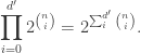
The right-hand size is a polynomial of degree \le d':=n/2+\log ^{d}(cs). The number of such polynomials is the number of possible choices for each monomial of degree i, for any i up to the degree. This number is

\begin{aligned} \prod _{i=0}^{d'}2^{{n \choose i}}=2^{\sum _{i}^{d'}{n \choose i}}. \end{aligned}

On the other hand, the number of possible functions f:S\to \{0,1\} is

\begin{aligned} 2^{|S|}. \end{aligned}

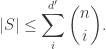
Since a polynomial computes at most one function, taking logs we have

\begin{aligned} |S|\le \sum _{i}^{d'}{n \choose i}. \end{aligned}

The right-hand side is at most 2^{n}(1/2+c\log ^{d}(s)/\sqrt {n}), since each binomial coefficient is \le c2^{n}/\sqrt {n}.

On the other hand, |S|\ge 0.9\cdot 2^{n}.

Combining this we get

\begin{aligned} 0.9\cdot 2^{n}\le 2^{n}(1/2+c\log ^{d}(s)/\sqrt {n}). \end{aligned}

This implies

\begin{aligned} 0.4\le c\log ^{d}(s)/\sqrt {n}, \end{aligned}

proving the theorem. QED

Exercise 10.6. Explain why Theorem 10.4 holds even if the circuits have Parity gates (in addition to Or and And gates).

[1]   Amir Abboud, Arturs Backurs, and Virginia Vassilevska Williams. Tight hardness results for LCS and other sequence similarity measures. In Venkatesan Guruswami, editor, IEEE 56th Annual Symposium on Foundations of Computer Science, FOCS 2015, Berkeley, CA, USA, 17-20 October, 2015, pages 59–78. IEEE Computer Society, 2015.

[2]   Leonard Adleman. Two theorems on random polynomial time. In 19th IEEE Symp. on Foundations of Computer Science (FOCS), pages 75–83. 1978.

[3]   Mikl�s Ajtai. \Sigma \sp {1}\sb {1}-formulae on finite structures. Annals of Pure and Applied Logic, 24(1):1–48, 1983.

[4]   Mikl�s Ajtai. A non-linear time lower bound for boolean branching programs. Theory of Computing, 1(1):149–176, 2005.

[5]   Eric Allender. A note on the power of threshold circuits. In 30th Symposium on Foundations of Computer Science, pages 580–584, Research Triangle Park, North Carolina, 30 October–1 November 1989. IEEE.

[6]   Eric Allender. The division breakthroughs. Bulletin of the EATCS, 74:61–77, 2001.

[7]   Eric Allender and Michal Koucký. Amplifying lower bounds by means of self-reducibility. J. of the ACM, 57(3), 2010.

[8]   Noga Alon, Oded Goldreich, Johan H�stad, and Ren� Peralta. Simple constructions of almost k-wise independent random variables. Random Structures & Algorithms, 3(3):289–304, 1992.

[9]   Dana Angluin and Leslie G. Valiant. Fast probabilistic algorithms for hamiltonian circuits and matchings. J. Comput. Syst. Sci., 18(2):155–193, 1979.

[10]   Sanjeev Arora, Carsten Lund, Rajeev Motwani, Madhu Sudan, and Mario Szegedy. Proof verification and the hardness of approximation problems. J. of the ACM, 45(3):501–555, May 1998.

[11]   Arturs Backurs and Piotr Indyk. Edit distance cannot be computed in strongly subquadratic time (unless SETH is false). SIAM J. Comput., 47(3):1087–1097, 2018.

[12]   Kenneth E. Batcher. Sorting networks and their applications. In AFIPS Spring Joint Computing Conference, volume 32, pages 307–314, 1968.

[13]   Paul Beame, Stephen A. Cook, and H. James Hoover. Log depth circuits for division and related problems. SIAM J. Comput., 15(4):994–1003, 1986.

[14]   Paul Beame, Michael Saks, Xiaodong Sun, and Erik Vee. Time-space trade-off lower bounds for randomized computation of decision problems. J. of the ACM, 50(2):154–195, 2003.

[15]   Michael Ben-Or and Richard Cleve. Computing algebraic formulas using a constant number of registers. SIAM J. on Computing, 21(1):54–58, 1992.

[16]   Samuel R. Buss and Ryan Williams. Limits on alternation trading proofs for time-space lower bounds. Comput. Complex., 24(3):533–600, 2015.

[17]   Lijie Chen and Roei Tell. Bootstrapping results for threshold circuits “just beyond” known lower bounds. In Moses Charikar and Edith Cohen, editors, Proceedings of the 51st Annual ACM SIGACT Symposium on Theory of Computing, STOC 2019, Phoenix, AZ, USA, June 23-26, 2019, pages 34–41. ACM, 2019.

[18]   Richard Cleve. Towards optimal simulations of formulas by bounded-width programs. Computational Complexity, 1:91–105, 1991.

[19]   Stephen A. Cook. A hierarchy for nondeterministic time complexity. J. of Computer and System Sciences, 7(4):343–353, 1973.

[20]   L. Csanky. Fast parallel matrix inversion algorithms. SIAM J. Comput., 5(4):618–623, 1976.

[21]   Lance Fortnow. Time-space tradeoffs for satisfiability. J. Comput. Syst. Sci., 60(2):337–353, 2000.

[22]   Aviezri S. Fraenkel and David Lichtenstein. Computing a perfect strategy for n x n chess requires time exponential in n. J. Comb. Theory, Ser. A, 31(2):199–214, 1981.

[23]   Michael L. Fredman and Michael E. Saks. The cell probe complexity of dynamic data structures. In ACM Symp. on the Theory of Computing (STOC), pages 345–354, 1989.

[24]   Anka Gajentaan and Mark H. Overmars. On a class of {O}(n^2) problems in computational geometry. Comput. Geom., 5:165–185, 1995.

[25]   M. R. Garey and David S. Johnson. Computers and Intractability: A Guide to the Theory of NP-Completeness. W. H. Freeman, 1979.

[26]   K. G�del. �ber formal unentscheidbare s�tze der Principia Mathematica und verwandter systeme I. Monatsh. Math. Phys., 38, 1931.

[27]   Oded Goldreich. Computational Complexity: A Conceptual Perspective. Cambridge University Press, 2008.

[28]   Raymond Greenlaw, H. James Hoover, and Walter Ruzzo. Limits to Parallel Computation: P-Completeness Theory. 02 2001.

[29]   David Harvey and Joris van der Hoeven. Integer multiplication in time O(n\mathrm {log}\, n). Annals of Mathematics, 193(2):563 – 617, 2021.

[30]   F. C. Hennie. One-tape, off-line turing machine computations. Information and Control, 8(6):553–578, 1965.

[31]   Fred Hennie and Richard Stearns. Two-tape simulation of multitape turing machines. J. of the ACM, 13:533–546, October 1966.

[32]   John E. Hopcroft, Wolfgang J. Paul, and Leslie G. Valiant. On time versus space. J. ACM, 24(2):332–337, 1977.

[33]   Russell Impagliazzo and Ramamohan Paturi. The complexity of k-sat. In IEEE Conf. on Computational Complexity (CCC), pages 237–, 1999.

[34]   Russell Impagliazzo, Ramamohan Paturi, and Michael E. Saks. Size-depth tradeoffs for threshold circuits. SIAM J. Comput., 26(3):693–707, 1997.

[35]   Russell Impagliazzo, Ramamohan Paturi, and Francis Zane. Which problems have strongly exponential complexity? J. Computer & Systems Sciences, 63(4):512–530, Dec 2001.

[36]   Russell Impagliazzo and Avi Wigderson. \mathit {P} = \mathit {BPP} if E requires exponential circuits: Derandomizing the XOR lemma. In 29th ACM Symp. on the Theory of Computing (STOC), pages 220–229. ACM, 1997.

[37]   Richard M. Karp and Richard J. Lipton. Turing machines that take advice. L’Enseignement Math�matique. Revue Internationale. IIe S�rie, 28(3-4):191–209, 1982.

[38]   Kojiro Kobayashi. On the structure of one-tape nondeterministic turing machine time hierarchy. Theor. Comput. Sci., 40:175–193, 1985.

[39]   Kasper Green Larsen, Omri Weinstein, and Huacheng Yu. Crossing the logarithmic barrier for dynamic boolean data structure lower bounds. SIAM J. Comput., 49(5), 2020.

[40]   Leonid A. Levin. Universal sequential search problems. Problemy Peredachi Informatsii, 9(3):115–116, 1973.

[41]   Carsten Lund, Lance Fortnow, Howard Karloff, and Noam Nisan. Algebraic methods for interactive proof systems. J. of the ACM, 39(4):859–868, October 1992.

[42]   O. B. Lupanov. A method of circuit synthesis. Izv. VUZ Radiofiz., 1:120–140, 1958.

[43]   Wolfgang Maass and Amir Schorr. Speed-up of Turing machines with one work tape and a two-way input tape. SIAM J. on Computing, 16(1):195–202, 1987.

[44]   David A. Mix Barrington. Bounded-width polynomial-size branching programs recognize exactly those languages in NC^1. J. of Computer and System Sciences, 38(1):150–164, 1989.

[45]   Joseph Naor and Moni Naor. Small-bias probability spaces: efficient constructions and applications. SIAM J. on Computing, 22(4):838–856, 1993.

[46]   E. I. Nechiporuk. A boolean function. Soviet Mathematics-Doklady, 169(4):765–766, 1966.

[47]   Valery A. Nepomnjaščiĭ. Rudimentary predicates and Turing calculations. Soviet Mathematics-Doklady, 11(6):1462–1465, 1970.

[48]   NEU. From RAM to SAT. Available at http://www.ccs.neu.edu/home/viola/, 2012.

[49]   Christos H. Papadimitriou and Mihalis Yannakakis. Optimization, approximation, and complexity classes. J. Comput. Syst. Sci., 43(3):425–440, 1991.

[50]   Wolfgang J. Paul, Nicholas Pippenger, Endre Szemer�di, and William T. Trotter. On determinism versus non-determinism and related problems (preliminary version). In IEEE Symp. on Foundations of Computer Science (FOCS), pages 429–438, 1983.

[51]   Nicholas Pippenger and Michael J. Fischer. Relations among complexity measures. J. of the ACM, 26(2):361–381, 1979.

[52]   Alexander Razborov. Lower bounds on the dimension of schemes of bounded depth in a complete basis containing the logical addition function. Akademiya Nauk SSSR. Matematicheskie Zametki, 41(4):598–607, 1987. English translation in Mathematical Notes of the Academy of Sci. of the USSR, 41(4):333-338, 1987.

[53]   Omer Reingold. Undirected connectivity in log-space. J. of the ACM, 55(4), 2008.

[54]   J. M. Robson. N by N checkers is exptime complete. SIAM J. Comput., 13(2):252–267, 1984.

[55]   Rahul Santhanam. On separators, segregators and time versus space. In IEEE Conf. on Computational Complexity (CCC), pages 286–294, 2001.

[56]   Walter J. Savitch. Relationships between nondeterministic and deterministic tape complexities. Journal of Computer and System Sciences, 4(2):177–192, 1970.

[57]   Arnold Sch�nhage. Storage modification machines. SIAM J. Comput., 9(3):490–508, 1980.

[58]   Adi Shamir. IP = PSPACE. J. of the ACM, 39(4):869–877, October 1992.

[59]   Claude E. Shannon. The synthesis of two-terminal switching circuits. Bell System Tech. J., 28:59–98, 1949.

[60]   Victor Shoup. New algorithms for finding irreducible polynomials over finite fields. Mathematics of Computation, 54(189):435–447, 1990.

[61]   Alan Siegel. On universal classes of extremely random constant-time hash functions. SIAM J. on Computing, 33(3):505–543, 2004.

[62]   Michael Sipser. A complexity theoretic approach to randomness. In ACM Symp. on the Theory of Computing (STOC), pages 330–335, 1983.

[63]   Roman Smolensky. Algebraic methods in the theory of lower bounds for Boolean circuit complexity. In 19th ACM Symp. on the Theory of Computing (STOC), pages 77–82. ACM, 1987.

[64]   Larry Stockmeyer and Albert R. Meyer. Cosmological lower bound on the circuit complexity of a small problem in logic. J. ACM, 49(6):753–784, 2002.

[65]   Seinosuke Toda. PP is as hard as the polynomial-time hierarchy. SIAM J. on Computing, 20(5):865–877, 1991.

[66]   Alan M. Turing. On computable numbers, with an application to the entscheidungsproblem. Proc. London Math. Soc., s2-42(1):230–265, 1937.

[67]   Leslie G. Valiant. Graph-theoretic arguments in low-level complexity. In 6th Symposium on Mathematical Foundations of Computer Science, volume 53 of Lecture Notes in Computer Science, pages 162–176. Springer, 1977.

[68]   Leslie G. Valiant and Vijay V. Vazirani. NP is as easy as detecting unique solutions. Theor. Comput. Sci., 47(3):85–93, 1986.

[69]   Dieter van Melkebeek. A survey of lower bounds for satisfiability and related problems. Foundations and Trends in Theoretical Computer Science, 2(3):197–303, 2006.

[70]   Dieter van Melkebeek and Ran Raz. A time lower bound for satisfiability. Theor. Comput. Sci., 348(2-3):311–320, 2005.

[71]   N. V. Vinodchandran. A note on the circuit complexity of PP. Theor. Comput. Sci., 347(1-2):415–418, 2005.

[72]   Emanuele Viola. On approximate majority and probabilistic time. Computational Complexity, 18(3):337–375, 2009.

[73]   Emanuele Viola. On the power of small-depth computation. Foundations and Trends in Theoretical Computer Science, 5(1):1–72, 2009.

[74]   Emanuele Viola. Reducing 3XOR to listing triangles, an exposition. Available at http://www.ccs.neu.edu/home/viola/, 2011.

[75]   Emanuele Viola. Lower bounds for data structures with space close to maximum imply circuit lower bounds. Theory of Computing, 15:1–9, 2019. Available at http://www.ccs.neu.edu/home/viola/.

[76]   Emanuele Viola. Pseudorandom bits and lower bounds for randomized turing machines. Theory of Computing, 18(10):1–12, 2022.