
You’ve built a strategy that works. Great.
Now you build another one. Also works.
You put them both in your portfolio and assume the risk has been cut in half.
It hasn’t.
Not automatically, anyway.
Whether combining strategies actually reduces your risk or just gives you the illusion of diversification comes down almost entirely to one thing: correlation.
Get this right and your equity curve gets smoother, your drawdowns get shallower, and you can size up with more confidence.
What Correlation Actually Means in This Context
In trading, correlation describes how similarly two strategies behave over time. Specifically: when one strategy is losing money, what is the other one doing?
A correlation of +1.0 means they move together perfectly, up together, down together. A correlation of 0 means they’re completely independent. A correlation of -1.0 means they move in opposite directions, when one is losing, the other is gaining.
For portfolio purposes, lower correlation is almost always better. You want strategies that have their bad periods at different times. That’s the entire game.
But if you calculate the total correlation with two strategies for let’s say 10 years back in a backtest you will probably get a very high number if it’s between two profitable strategies because overtime they both move up and to the right, that’s why it’s specifically useful to use drawdown correlation in systematic trading and not the performance correlation.
The basic steps to calculate drawdown correlation:
Calculate the running drawdown for each strategy at every point in time meaning how far each strategy is currently sitting below its peak equity at that date
You now have two drawdown series (e.g. Strategy A is -8%, Strategy B is -3% on day X)
Run a standard Pearson correlation on those two drawdown series instead of on the return series
However, there are purposes for using very similar strategies as well, let’s say you only have a single mean-reversion strategy on Nasdaq, if that strategy would fail and eventually start to decay rapidly you want to be able to turn that strategy off and replace it with a similar type but another strategy that works. For this reason I actually believe similar strategies have a purpose as well as long as they are robust.
A Simple Example: The Same Strategy Twice
Imagine you run a mean-reversion strategy on the S&P 500. It goes through a rough time in a trending market, say a sustained uptrend where every pullback just keeps going. That’s a normal rough patch for that type of strategy.
Now imagine you add a second strategy, also mean-reversion, also on a major equity index. When the S&P is trending hard, European indices probably are too. Both strategies hit their rough patches at the same time. Your drawdown is just as deep as if you’d run one strategy. You’ve doubled your capital at risk but got almost nothing in return for it.
High correlation between your strategies means your worst periods stack on top of each other. The losses don’t cancel, they compound.
Join 7,500+ traders learning systematic trading. Premium members get full access to all my Substack strategies.
What Good Diversification Looks Like
Contrast that with pairing a mean-reversion strategy with a trend-following strategy. They have fundamentally different requirements from the market. Mean-reversion needs range-bound, choppy conditions. Trend-following needs sustained directional movement.
In a trending market, your mean-reversion strategy struggles, but your trend-following strategy thrives. In a choppy, directionless market, the opposite is true. The bad periods don’t overlap. Your overall equity curve smooths out considerably.
The total return of the portfolio isn’t necessarily higher, but the journey to get there is much more consistent, and the maximum drawdown is often dramatically lower. That matters enormously when you’re trying to stay in the game long enough for the edge to play out.
How to Actually Measure It
The standard way is to calculate the Pearson correlation coefficient between the daily or weekly returns of each strategy. In ProRealTime, you can export your strategy equity data and run this in a spreadsheet/python.
A rough guide for interpreting the results:
0.7 to 1.0: High correlation. These strategies are too similar. Adding the second one adds risk, not diversification.
0.3 to 0.7: Moderate correlation. Some benefit, but limited.
0.0 to 0.3: Low correlation. Solid diversification. This is what you’re aiming for.
Below 0: Negative correlation. Excellent. Each strategy partially hedges the other.

Don’t stop at pairs either. Once you have three or more strategies, build a full correlation matrix, every strategy against every other. Something might look uncorrelated with Strategy A but be highly correlated with Strategy B that’s already in your portfolio. You need the full picture.
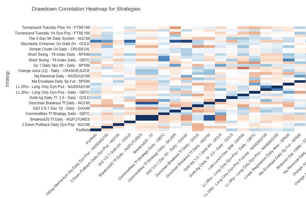
Here’s a simple example with three strategies. Strategy A and Strategy B have a correlation of 0.12, basically independent. Strategy B and Strategy C come in at 0.09, also well diversified. But Strategy A and Strategy C have a correlation of 0.68, which is high. They’re probably built on similar logic or trading similar markets. Adding C to a portfolio that already has A gives you very little real diversification, even though C looks fine when measured against B in isolation. That’s the kind of hidden overlap you only catch when you check every pair, not just the obvious ones.
What Drives Correlation, And How to Reduce It
Two strategies tend to be highly correlated when they share similar logic, similar markets, or similar time horizons. The most common mistake is building slight variations of the same strategy, tweaking an entry rule here, adjusting a filter there, and thinking that counts as diversification. It doesn’t. If the underlying logic is the same, the correlation will be high regardless of the surface-level differences.
The most effective ways to genuinely reduce correlation: trade different strategy types (mean-reversion vs trend-following vs breakout), trade different markets (equities vs commodities vs fixed income), trade different timeframes (intraday vs daily vs weekly), and mix long-biased and short-biased logic. You don’t need all of these. Even one meaningful structural difference can bring correlation down significantly.
The Part Most People Miss: Correlation Isn’t Static
This is where a lot of portfolio builders get caught off guard.
Correlation between strategies can shift significantly depending on market regime. Two strategies that look uncorrelated on average might suddenly start moving together when conditions change. This is one of the most important things to understand before trusting your correlation numbers.
A concrete example: during a low-volatility, steadily trending bull market, a trend-following equity strategy and a mean-reversion equity strategy might show low correlation, they’re taking turns performing well. But during a sharp market crash, both can struggle simultaneously. The trend-follower gets whipsawed by the speed of the move. The mean-reversion strategy keeps buying “cheap” as prices fall further. Suddenly two strategies that looked diversified are both deep in drawdown at the same time, in exactly the moment you need diversification most.
This is sometimes called correlation breakdown and it’s particularly common during high-stress market environments like crashes, liquidity crises, or sharp volatility spikes.
Rather than just calculating one correlation number across your entire backtest period, split your backtest into regimes and calculate correlation separately for each: low volatility periods (e.g. VIX below 15), high volatility periods (e.g. VIX above 25), trending markets (e.g. price consistently above a 200-day moving average), and choppy/range-bound markets.
If your strategies show low correlation across all of these regimes, you have genuine diversification. If they look uncorrelated on average but converge during high-volatility periods, you have a hidden concentration risk, one that will show up at exactly the wrong time.
The safest portfolio isn’t one with the best average correlation. It’s one with the most stable correlation across all conditions.
The Practical Takeaway
When you add a new strategy to your portfolio, the first question shouldn’t be “does it have good returns?” It should be “when does it lose money, does that overlap with what I’m already running and does that hold across different market conditions?”
A mediocre strategy that’s genuinely uncorrelated with your existing portfolio, across regimes and not just on average, can add more value than a great strategy that moves with everything else you’re running. The returns get averaged. But the risk reduction is real and it’s there when you need it the most.
Building a good portfolio isn’t about stacking winners. It’s about stacking strategies that fail at different times and verifying that’s actually true before you put money on it.
The Algomatic Trading database gives you a growing library of fully coded, tested strategies across different markets and logic types. Built specifically so you can combine them into a portfolio with confidence. If you’re serious about building something systematic that holds up, the full database is available for premium members.
Comments
Nothing yet. Say the first thing.
Sign in to join the conversation.