Toto-2.0: Time Series Forecasting Finally Scales Like LLMs

Toto-2.0 sets a new bar for time series foundation models.

In previous articles, we covered Toto-2.0 through practical tutorials, sharing a Retail Forecasting walkthrough and exploring the BOOM and TIME benchmarks.

Now it’s time to look at the model itself.

Toto-1.0 was released last year. There was also an even earlier version, a 2024 paper[1] without model weights that appeared during the first wave of foundation models for time series, together with Chronos-1 and MOIRAI-1.

Toto-2 does something none of the other foundation models have done. It scales. The authors released 5 model sizes (4m, 22m, 313m, 1B, 2.5B), and every size improves on the one below it. Toto-2.0 also takes the top spot on all public forecasting benchmarks (for now!).

In this article, we’ll dive into Toto-2.0’s architecture, the new optimizer (NorMuon), and the hyperparameter pipeline that makes the scaling work.

What makes Toto-2.0 stand out? A few design choices stacked together:

• Contiguous Patch Masking (CPM) replaces autoregressive decoding with a single parallel forward pass.

• Arcsinh normalization keeps small fluctuations visible while compressing extreme spikes - perfect for sparse data.

• NorMuon optimizer handles the sign-valued gradients of pinball loss far better than AdamW.

• u-µP hyperparameter transfer tunes settings once on a 10M proxy model and reuses them across all 5 target sizes.

All these choices push Toto-2.0 to the top of every public benchmark. Let's get started!

Subscribe to AI Horizon Forecast, a newsletter focusing on time series and hype-free AI research. Also, check the following notebooks on Toto-2:

• Edge Cases with Toto 2 - and how to avoid them - Project 33

• TIME & Boom datasets (Sparse) - Project 30/ Project 31

• Retail Forecasting / Energy demand forecasting - Project 29 / Project 32
  

Toto 2.0 is Datadog’s decoder-only foundation model built for multivariate zero-shot time-series forecasting.

Here are the key properties (we saw these briefly in the previous article):

• Decoder-only architecture: A patched transformer that alternates time-axis and variate-axis attention (kept from Toto-1). It supports variable context lengths and accepts future-known covariates.

• u-µP scaling: Hyperparameters are tuned once on a tiny 10M proxy model and transfer directly to the 2.5B version, without any expensive retuning at each scale.

• Near-instant inference with CPM: Contiguous Patch Masking lets the model generate long horizons (great performance up to ~768 steps) in a single parallel forward pass, instead of slow autoregressive decoding.

• Probabilistic forecasting: A quantile head trained with pinball loss produces both point forecasts and uncertainty estimates.

• State of the art: Top spots on BOOM, GIFT-Eval, and the contamination-resistant TIME benchmark. Released as open-weights under Apache 2.0.

Now let's explore in detail how Toto-2.0 works.

Toto-2.0 keeps the decoder-only patched transformer from Toto-1.0:

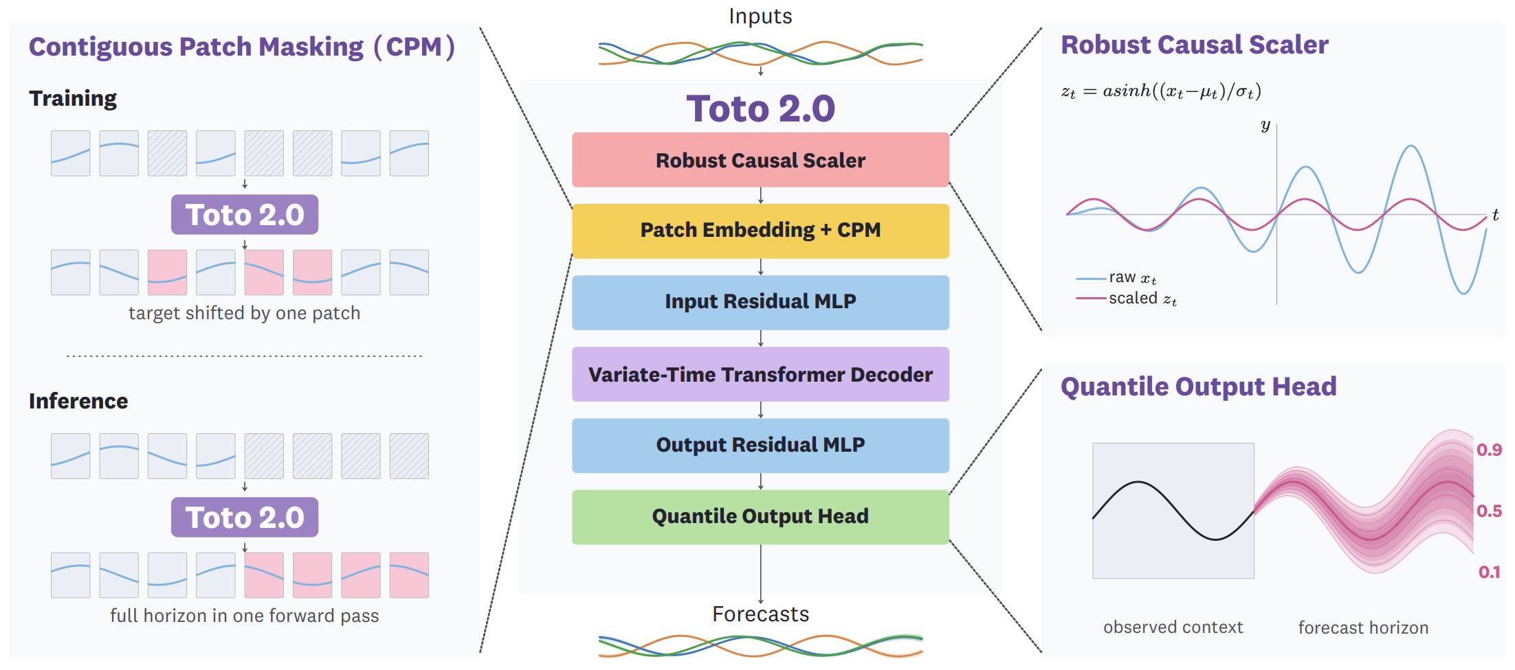
The data flow is the following:

1. Raw inputs pass through a robust causal scaler with arcsinh normalization.

2. Then the inputs are split into non-overlapping patches (of size 32, down from 64 in Toto-1) and then embedded. CPM is also applied during training, masking random patches.

3. These patches flow through a stack of Transformer blocks that alternate between time-axis attention (causal, across time) and variate-axis attention (full, across all time series in the batch).

4. A residual MLP projects patches into the model (latent) dimension.

5. The variate-time transformer decoder processes them.

6. An output residual MLP feeds the quantile head, which predicts the final forecasts (the 9 quantiles). Toto-2.0 doesn’t separately produce the mean (point forecast) and 9 quantiles - instead, the point forecast is the median (5th quantile)

The most important changes from Toto-1.0 are arcsinh normalization, CPM, the quantile head, and NorMuon. Let's look at each.

This change is borrowed from Chronos and works beautifully for all TSFMs.

Unlike logarithmic scaling, arcsinh behaves linearly near zero. This preserves the small differences that show up in sparse and intermittent time series. For large values, it behaves like a logarithm, compressing extreme spikes (Figure 2).

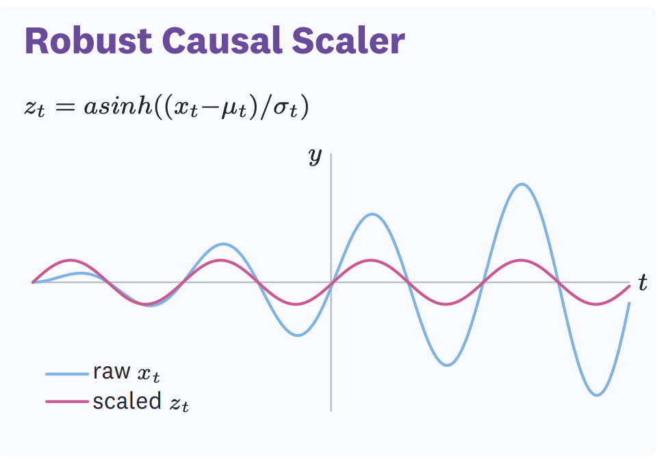
The combination is exactly what foundation models need. Small differences stay visible, large outliers stay manageable, and the model can learn from datasets that span many orders of magnitude during pretraining.

Toto-1.0 used a Student-T mixture model (SMM) for probabilistic forecasts. It worked well at Toto-1.0’s scale, but as the models grew larger, the SMM became numerically unstable. It diverges when predictions approach zero because of the variance term in its normalization.

Toto-2.0 replaces SMM with a simple quantile head. For each future timestep, the model predicts 9 quantile levels {0.1, 0.2, ..., 0.9}, trained with pinball loss. This approach is now standard among leading foundation models like Chronos-2, Moirai-2, and TimesFM 2.5. We discussed the reason for this here.

To prevent quantile crossing, predictions are sorted before being returned at inference.

Toto-1.0 generated forecasts autoregressively, one patch at a time. A 1024-step horizon required up to 16 sequential forward passes, and errors compounded across them.

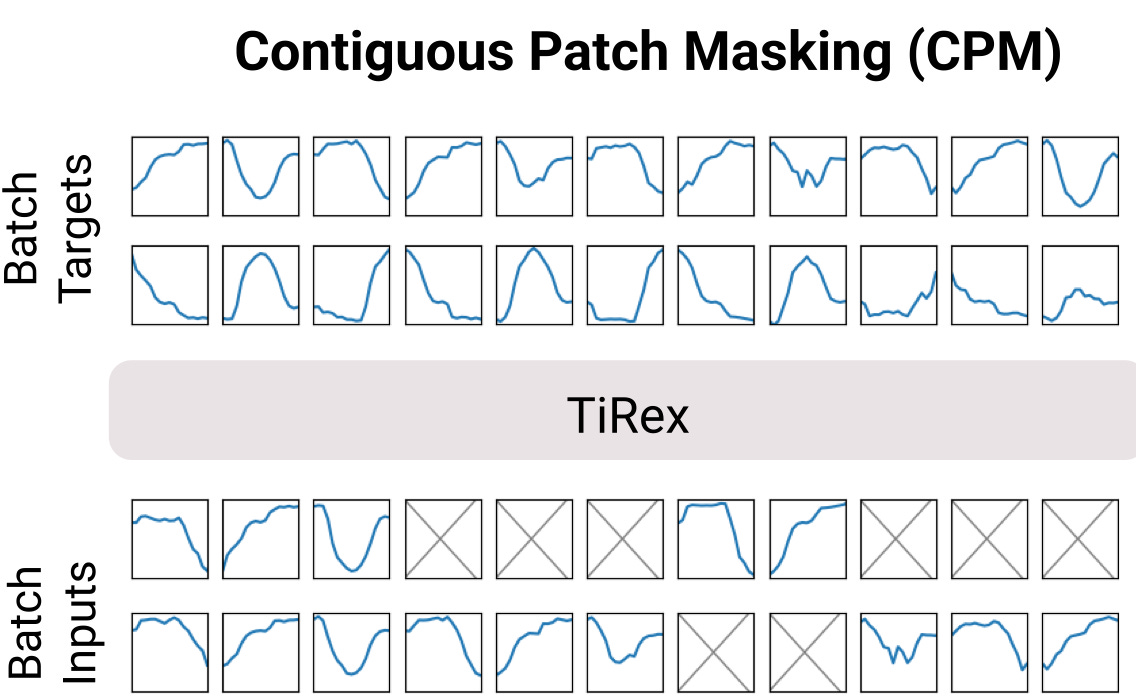
CPM (Figure 3), adapted from the TiRex model, fixes this. During training, the model learns to predict multiple future patches at once by masking variable-length contiguous spans of the input. At inference, the entire forecast horizon is filled with mask tokens and decoded in a single forward pass.

The result is blazingly fast inference. Single-pass decoding generally remains stable up to a ~768-step horizon on synthetic multi-scale signals. For longer horizons, Toto-2 supports block decoding, generating the forecast in segments while reusing the KV cache.

We covered CPM in detail in my TiRex article - check it for more info if you are not familiar with CPM, because we will later discuss CPM’s parameters!

Most TSFMs rely on Mean Squared Error (MSE), where the mathematical penalty scales with the size of the mistake:

And its gradient is:

Since the gradient is directly proportional to the error, the optimizer gets a clear, magnitude-bearing signal of how big a corrective step to take. This gives training a wide dynamic range. Massive updates when predictions are way off, smaller steps when they are close.

Toto-2.0 shifts to pinball loss for quantile forecasting, which fundamentally changes how the model registers its errors. The pinball loss is:

And its gradient is:

Visually, the pinball loss looks like a V (or a skewed V) made of straight lines. The derivative of a straight line is always a constant. Because of this geometric shape, the gradient follows three strict rules:

• If you under-forecast, the gradient is exactly −τ.

• If you over-forecast, the gradient is exactly 1−τ.

• If you are perfectly accurate, it is 0.

Under pinball loss, the gradient only tells the model the direction it was wrong and the quantile it is targeting. It completely loses the magnitude information. A 1-unit miss and a 1000-unit miss produce the same gradient magnitude.

The authors call these “sign-valued gradients” because the slope is dictated almost entirely by the sign of the error.

This lack of magnitude information breaks AdamW, the default optimizer for most modern deep learning models. Adam tracks the fluctuating variance of gradients for every single weight in isolation to calculate an adaptive step size. With pinball gradients essentially constant, Adam’s internal variance tracker flatlines.

Thinking the gradients are perfectly stable, the optimizer stops meaningfully adjusting the learning pace. Since Adam only sees one parameter at a time, and those individual gradients never change size, it gets stuck operating in a severely narrowed dynamic range. It knows which direction to move to correct the forecast, but it has lost the mathematical context required to determine how far to jump.

NorMuon solves this optimization crisis by fundamentally changing where the engine looks for its magnitude information. Instead of isolating single weights as Adam does, NorMuon zooms out and calculates variance across an entire neuron, which corresponds to a full row of weights in the matrix.

Even though individual gradients are constants, the collective pattern of updates across that entire row reveals how active or important that specific neuron is. By normalizing the step size against the whole row, NorMuon restores the model’s ability to efficiently adapt its learning pace.

Before getting into the details, let’s cover the basics, assuming you’ve never encountered u-µP before.

Besides, this is the secret sauce behind Toto-2.0's scaling, and it's a technique I myself hadn't encountered before.

When training a neural network, you need to choose a bunch of settings before training even starts - the learning rate, weight decay, how momentum behaves, and so on. These are called hyperparameters. The standard approach is to try many combinations, measure which performs best on a validation set, and use those.

The problem is that when you change model size, specifically model width, the optimal settings change too. For example, the optimal learning rate can shift by an order of magnitude between a small and a large model. So if you’re training 5 models of different sizes, you’d normally need 5 separate searches. With each target model taking days to train, that’s a lot of wasted compute.

µP (Maximal Update Parametrization) solves this with a mathematical reparametrization of each weight. Under µP, the learning dynamics become independent of model width. A setting that works for a small model works for a large one too. u-µP is the “unit-scaled” variant, simpler to implement and better suited to decoder-only architectures.

With u-µP, you tune hyperparameters on a cheap, tiny model (the “proxy”), then transfer those settings directly to every larger size. No returning.

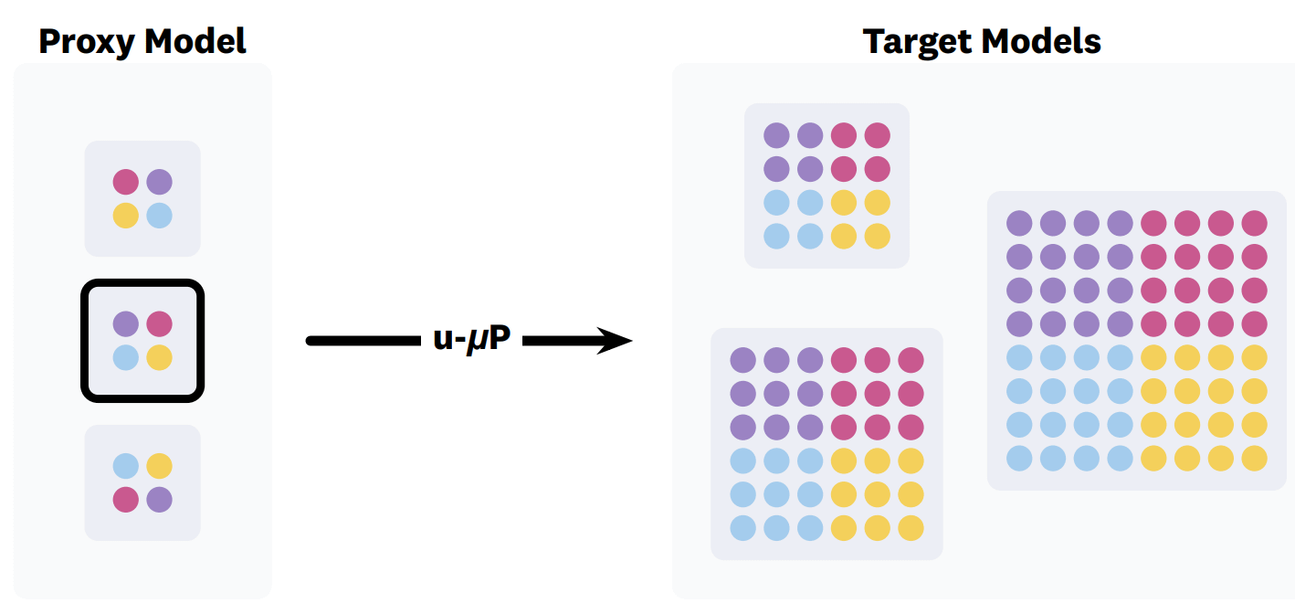
A few important clarifications about how this transfer works:

• The proxy is only used to find hyperparameters, not weights. Once the search is complete, the proxy’s learned weights are discarded. Each target size (4m, 22m, 313m, 1B, 2.5B) is then trained from scratch using the hyperparameters found by the proxy.

• What transfers is the configuration, not the parameters: learning rate, weight decay, momentum, decay schedule, as well as architecture choices like attention placement and data mixture.

• Width, depth, and number of attention heads are different per model size. Only the fundamental hyperparameters stay the same. The bigger models get more layers, wider embeddings, and more attention heads.

Now we need a search procedure. Even at proxy scale, the joint search space spans 17 continuous and several categorical dimensions, about 10^19 configurations under a modest grid. Exhaustive search is impossible.

The authors split the process into 4 sequential rounds:

1. Architecture: Sweep attention normalization, the placement and frequency of variate-axis attention layers, bias terms, and CPM parameters.

2. Data mixture: Find the best ratio of internal, synthetic, and public data sources.

3. Optimizer: Tune learning rate, weight decay, and momentum terms for NorMuon and AdamW.

4. Decay schedule: Sweep the length and shape (linear or 1-sqrt) of the learning rate decay.

Each round freezes the best configuration found in the previous round and only searches over the new group. For example, once Round 1 picks the best architecture, that architecture is fixed for Round 2. Then Round 2 picks the best data mixture, which is fixed for Round 3, and so on.

This sequential design follows a natural dependency chain. Architecture and data shape the loss landscape, the optimizer must adapt to that landscape, and the decay schedule is tuned downstream of the optimized stable regime. You cannot pick a good learning rate without knowing the architecture, and you cannot tune the decay schedule without knowing how the optimizer behaves in steady state.

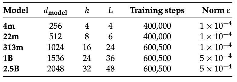
The Toto-2.0 proxy is a 10M-parameter model (L=12, dmodel​=256, h=4), where:

• L is the number of transformer layers (depth)

• dmodel​ is the embedding dimension (width)

• h is the number of attention heads.

Each sweep trial trains for 30000 steps at the same batch size used for target models. A trial finishes in hours, instead of the days a target model would need. Here’s the diagram of the 4 rounds and what was tested each time:

After the 4 rounds, the best configuration was:

• Architecture: PerDimScale attention, variate-axis attention layer placed last in the stack, CPM with cmax⁡=16 and pmax⁡=0.4.

• Data mixture: 42.5% Datadog observability + 57.5% synthetic data. Public data was excluded entirely.

• Optimizer: NorMuon at η=0.65, AdamW at η=0.012 for input/output projections, both with some weight decay.

• Schedule: Linear decay over 10500 steps.

This single configuration is then applied to all 5 target sizes (4m, 22m, 313m, 1B, 2.5B). Only dmodel, number of transformer layers, and number of attention heads change between them. The values of the target models (Toto-2.0 final variants) are shown in Table 1 below:

Remember, every target model still trains from scratch!

Quick note on pretraining data before we look at numbers.

Unlike most foundation models, Toto-2.0 doesn’t see any public time series data during pretraining. Its 5.04T data points (for the 3 largest sizes) come from Datadog’s internal observability metrics (CPU utilization, memory, request latency, error rates) and synthetic data generated with TempoPFN’s prior-data-fitted network framework.

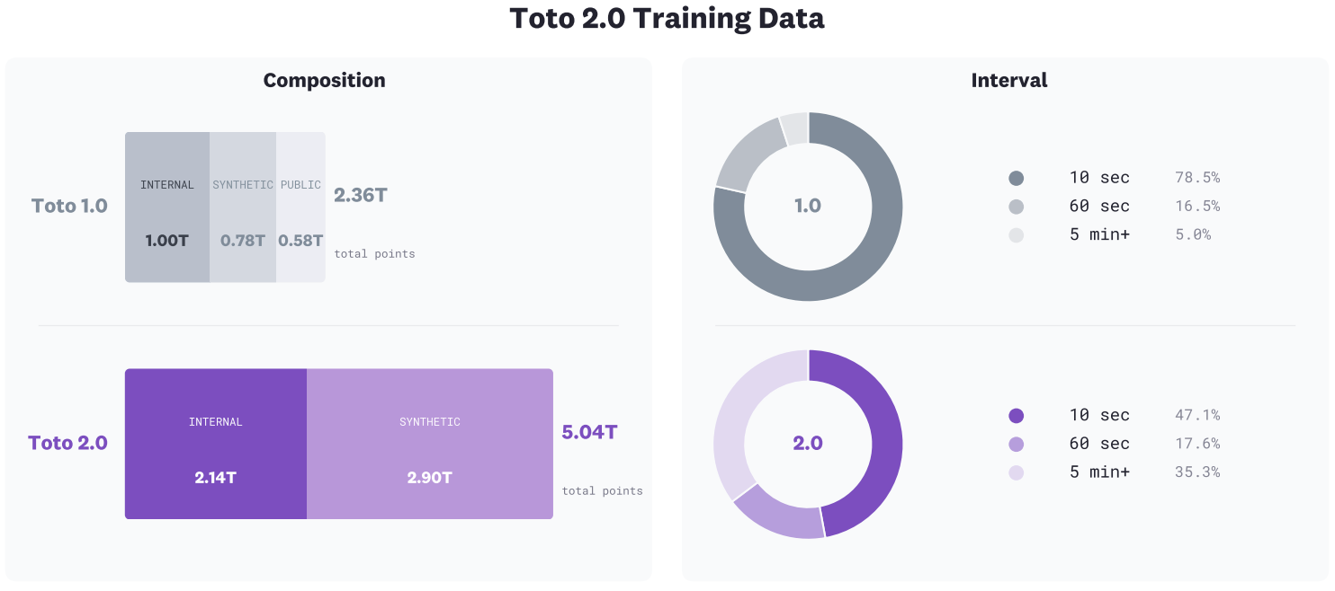
Public data only enters the recipe during finetuning, making up 45% of the mix for the 2.5B-FT variant. This makes Toto-2.0’s results on public benchmarks more impressive: the base models have never seen any public evaluation domain.

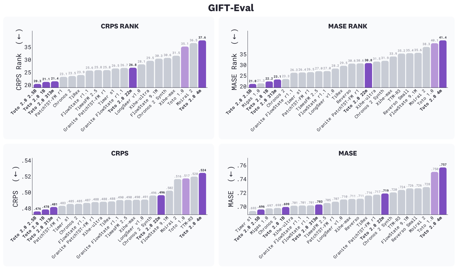
GIFT-Eval covers 97 evaluation tasks from 23 base datasets across energy, retail, weather, and finance.

Key takeaways:

• Toto-2’s three largest sizes (313m, 1B, 2.5B) take the top 3 spots on CRPS rank: 20.3, 21.1, and 21.4, respectively.

• There’s a 1.7-point gap from the 313m to the next best foundation model, PatchTST-FM r1 at 23.1.

• Chronos-2, a strong competitor, sits at 23.5.

• The 22m at 26.8 beats Toto-1 (35.1) by more than 8 points.

• Every Toto-2 size improves on the one below it.

• Toto-1 is a 1st-generation TSFM - notice that all 2nd-generation TSFMs surpass it, demonstrating the rapid progress of these models!

Be careful! The proxy model's hyperparameters were optimized against the GIFT-Eval validation set. This is not direct data leakage (the model never sees GIFT-Eval data during training), but the hyperparameter choice is informed by GIFT-Eval performance. Worth keeping in mind when comparing to models that don't tune on GIFT-Eval. In our Electricity tutorial (Project 32), we resample to a 6H frequency to remove any doubt for data leakage!

When the leaderboard is opened up to finetuned and ensembled variants, Toto-2 takes both top spots:

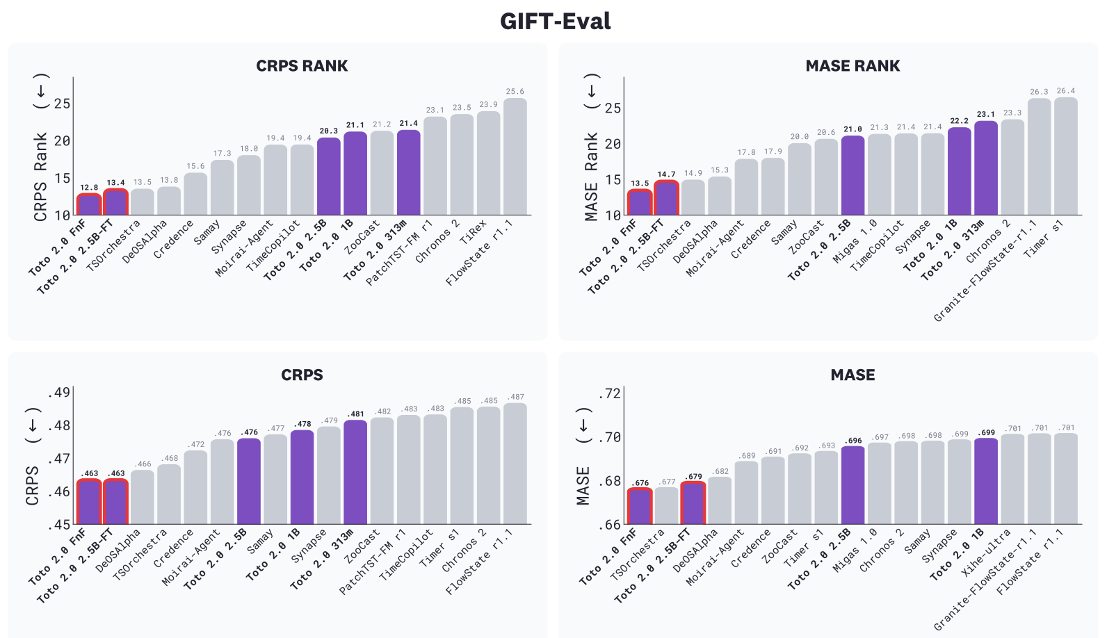
• Toto 2.0 FnF: An ensemble using XGBoost as the meta-learner across 10 foundation models (all 5 Toto-2 sizes plus Chronos-2, TimesFM 2.5, TiRex, FlowState, and PatchTST-FM r1). Ranks #1 on every metric.

• Toto 2.0 2.5B-FT: The 2.5B base model finetuned on a mix including GIFT-Eval’s official train split. Ranks #2 on the rank metrics.

The most interesting finding is what happens inside the ensemble. When the FnF meta-learner is free to weight everything available to it, the Toto-2.0 family gets 39% of the assigned weight on average, more than any other source.

BOOM evaluates forecasting on observability metrics: CPU utilization, memory usage, request latency, and error rates.

These are the signals production monitoring systems care about. As a Datadog-built benchmark(released when Toto-1.0 was released last year), BOOM plays to Toto-2’s strengths.

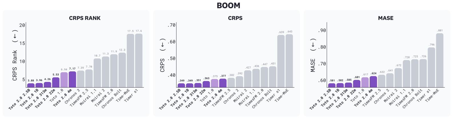
We notice that:

• Every Toto-2.0 size sits on the Pareto frontier of BOOM. At any parameter count, no other foundation model produces better forecasts. (Figure 9)

• The three largest sizes lead with CRPS ranks of 3.88 (2.5B), 3.96 (1B), and 4.26 (313m).

• The 22m at 5.53 beats Toto-1 (6.94) with roughly 7× fewer parameters.

• The 4m at 7.17 is competitive with Toto-1.0 and Chronos-2 (7.39) despite being ~38× smaller. A strong option for edge deployment.

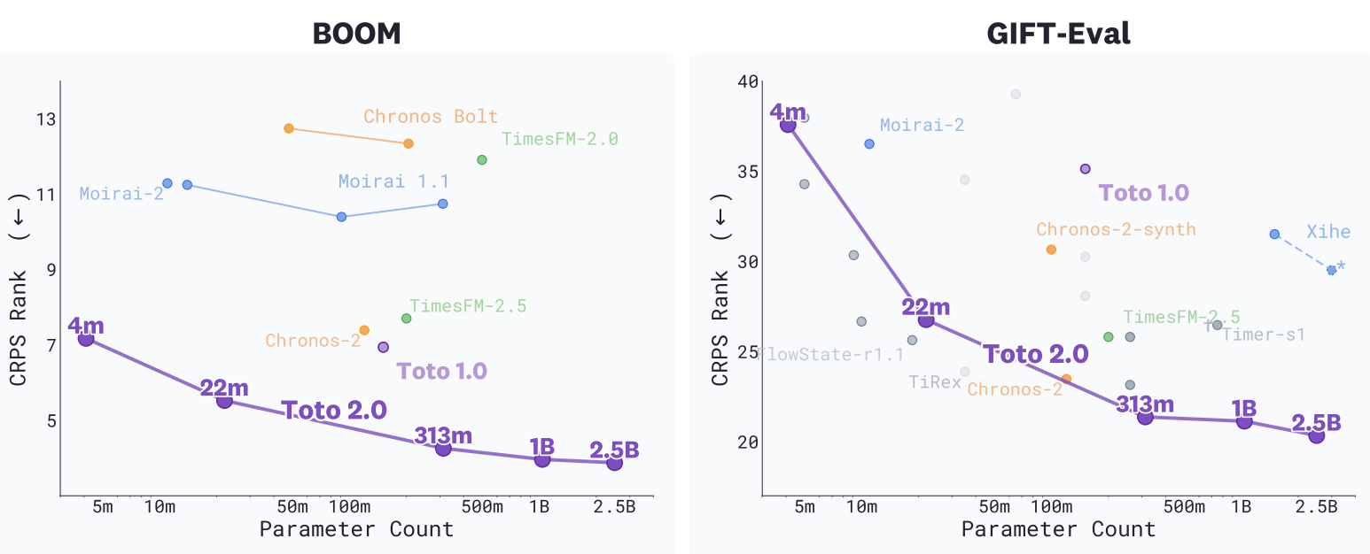
Figure 9 makes the scaling claim visually obvious. Toto-2.0 is the only family where every size sits on or near the frontier of both benchmarks.

Feel free to check the paper for more details. There’s also the TIME benchmark evaluation, which I don’t discuss here - and where the Toto-2.0 variants again achieved top positions

CPM doesn't just improve forecast quality. It makes Toto-2.0 dramatically faster.

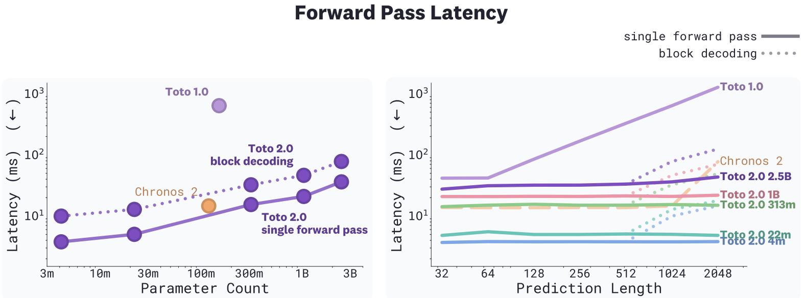
A 1024-step forecast takes Toto-1.0 up to 16 autoregressive steps. Toto-2.0 does it in a single forward pass. The 313m runs at roughly the same latency as Chronos-2 (120M parameters), despite being more than twice the size.

At 4096-step horizons, even the 2.5B in single-pass mode remains faster than Chronos-2.

For really long horizons, the authors test Toto-2.0 on synthetic multi-scale sinusoids at 2048, 4096, and 8192 timesteps. The training context is 4096.

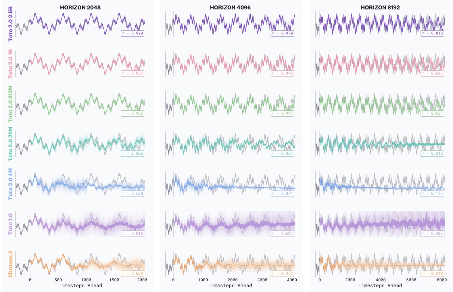
The pattern is striking:

• 4m: Captures short-range patterns but collapses past its training context.

• 22m: Holds longer but degrades by 4096 steps.

• 313m: Stable through 4096 but loses structure beyond.

• 1B: Maintains the underlying pattern across all 3 horizons.

• 2.5B: Most accurate of all.

Toto-1 and Chronos-2 both lose coherence well before the 1B model, despite Chronos-2 being trained on longer sequences. Scale really does matter for long-horizon coherence.

Below are some limitations you need to know before using the model

1. Toto-2.0’s context length should be a multiple of the patch size(32)

2. Toto-2.0 does not support panel-data covariates (covariate-informed) like Chronos-2 and full channel mixing together. It works with global covariates (e.g., calendar features or macroeconomic indicators), but not with entity-specific covariates (e.g., country-specific holidays or store-specific promotions), since its channel mixing assumes that each covariate has the same meaning across all time series - unless we disable global mixing and each panel predicts using its own covariates. Don’t worry if you don’t get it, we'll discuss this in detail in our next article.

3. The released model doesn’t support fine-tuning - but the paper implies it does. Like Toto-1, this is something that might be added in the future

4. Toto-2.0 falls behind AutoTheta on the second-level frequency, ending a recent run where new TSFMs had consistently outperformed it at that granularity.

There are a few other limitations as well that we’ll discuss in our next article. If you want to take a peek, I already have a notebook on these, check Project 33

Toto-2.0 is a major step forward for time series foundation models.

Beyond taking the top spot on every public benchmark, it delivers something the field has been waiting for: clean, reliable scaling. Each of the 5 sizes improves on the one below it, and the largest model handles long horizons that break every competitor.

The 4 core design choices, CPM for single-pass inference, arcsinh for wide-range normalization, NorMuon for pinball loss training, and u-µP for hyperparameter transfer, each solve a real problem. Together, they push the model to the top.

Also, there is much debate about scaling laws in time series, and research presents conflicting evidence. Toto-2.0 shows scale is real, thanks to u-µP.

In the next and final article of the Toto-2 series, we will discuss some edge cases and how to take the model to the next level. Stay tuned!

Horizon AI Forecast is a reader-supported newsletter, featuring occasional bonus posts for supporters. Your support through a paid subscription would be greatly appreciated.

[1] Cohen et al. Toto: Time Series Optimized Transformer for Observability

[2] Cohen et al. Toto and BOOM unleashed: Datadog releases a state-of-the-art open-weights time series foundation model and an observability benchmark

[3] Khwaja et al. Toto 2.0: Time Series Forecasting Enters the Scaling Era

[4] Auer, Andreas; Podest, Patrick; Klotz, Daniel; Böck, Sebastian; Klambauer, Günter; Hochreiter, Sepp. TiRex: Zero‑Shot Forecasting Across Long and Short Horizons with Enhanced In‑Context Learning (May 2025).