
Time series foundation models are one of the biggest shifts in forecasting in the last 2 years.
They have real potential, and they can perform very well in the right setting.
But they also have weaknesses. A lot of online content I read focuses on the exciting parts and skips the issues that actually matter in practice, or they call things “limitations” when they really have straightforward workarounds.
In this article, we will take a technical, hype-free look at the true limits of time-series foundation models(TSFMs) and explore which ones can be addressed, which ones cannot, and which ones are still open problems.
Follow AI Horizon Forecast, a newsletter focusing on time series and hype-free AI research. Also, check the AI Projects accompanying this newsletter, including the latest project on TabICLv2!
Let’s start with the true challenges first.
Most foundation models are pretrained on a fixed objective.
In many cases, this is a mean-optimized regression loss like MSE, while models that support probabilistic forecasting use multi-quantile loss (MQL), typically with ~9 quantiles. A notable exception is Chronos-2, which is pretrained on 21 quantiles (0.01 to 0.99).
Early foundation models explored more flexible objectives. For example, MOIRAI-1 uses a mixture of distributions (Student’s t, log-normal, negative binomial, normal) instead of a single loss. This direction was later dropped in MOIRAI-2, which moved to a quantile-based objective. To the best of my knowledge, only Toto still uses a composite-style robust objective while remaining competitive.
The underlying assumption is that MSE or MQL is “good enough” and that a well-pretrained model can generalize across all cases. In practice, supervised models show the opposite: choosing the right loss function often makes a huge difference. If you want robustness to outliers, use Huber loss. For retail forecasting with non-negative counts, the negative-binomial likelihood is more appropriate, and if high skew + zero-inflated data are also present, use Tweedie.
Additionally, more advanced setups go even further. In global models, practitioners sometimes use asymmetric or weighted losses like WRMSSE, placing a higher weight on high-revenue products, or when over- and under-predictions are penalized differently.
So, there are 2 main issues regarding this category:
The sophistication of the loss function is lost when using a foundation model because you cannot change or adapt it after pretraining.
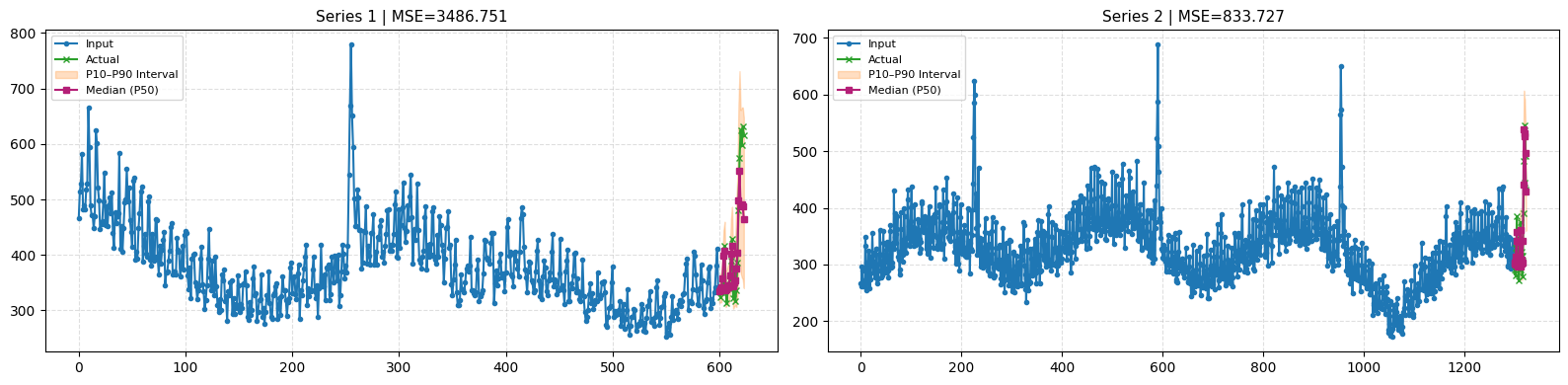
A smaller but practical issue appears on noisier, sparser datasets. Even when the target is strictly positive (e.g., sales), the model may still output negative values—especially in lower quantiles. This is rare, but it does happen.
How to fix this:
These challenges cannot be addressed directly—only mitigated through workarounds:
There is no way to change the loss function after pretraining. However, increasing the context length usually helps, as it gives the time series foundation model more visibility into the structure and peculiarities of the dataset. In practice, the model relies on the global inductive biases it learned during pretraining and adapts them to the longer context.
Another option is to fine-tune the model on your dataset. This helps align the model with the data’s behavior. You lose zero-shot capability, but this is typically a one-time cost. For example, in an energy forecasting task I tried with Chronos-2, the 10th quantile occasionally became negative despite strictly positive targets, but fine-tuning fixed the issue.
When time series foundation models first appeared, one pattern stood out: they struggled with higher-frequency data. In some cases, simple statistical models like AutoTheta even outperformed them.
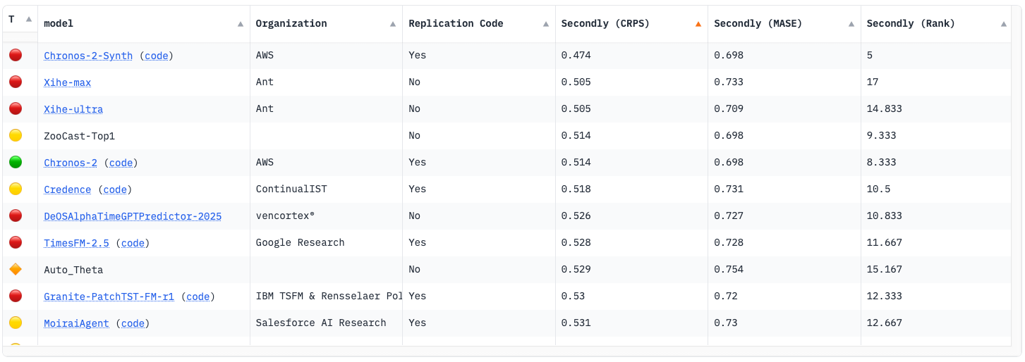
You can notice this at the GIFT-Eval benchmark, where only Chronos-2 and TimesFM-2.5 among the basic models manage to beat Auto Theta on the secondly frequency. As frequency decreases, foundation models become more competitive.
If we look under the hood, this behavior makes sense. Most time series foundation models process data using patching—a window of consecutive values mapped into a latent embedding, similar to tokens in LLMs.
However, patch size controls how information is aggregated, implicitly favoring certain frequencies. Larger patches smooth the signal and emphasize low-frequency components, while smaller patches preserve higher-frequency detail. For example, models like Chronos-2 and TimesFM use fixed patching schemes that tend to bias toward lower frequencies. This improves long-horizon forecasting and aligns with many real-world datasets—but introduces a temporal bias against high-frequency signals.
This effect is not just empirical—it has been formally analyzed in recent work [1], showing how patching induces frequency-dependent behavior:
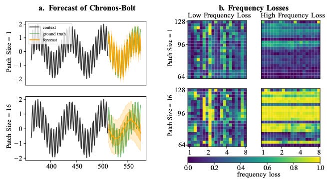
Chronos-1 is a special case. It effectively operates with patch size 1, preserving full resolution, but relies on quantization and cross-entropy training, which leads to different trade-offs compared to its patched successors.
Some models, like Moirai-1, attempt to address this by using multiple patch sizes tied to data frequency. In practice, this adds complexity, and newer models have largely moved away from this design:

What does this mean in practice?
Temporal bias is still implicit in current time series foundation models. While they have improved on higher frequencies, datasets with minutely or secondly granularity still favor strong statistical baselines—especially for short-term forecasting.
In other words, time series foundation models shine at structure and scale, but at very high frequencies, classic methods remain surprisingly challenging to beat (especially in short-term forecasting).
But what happens at lower frequencies? Do foundation models always have the upper hand?
Foundation models are often presented as plug-and-play tools that need no tuning and can be readily used to deliver decent predictions. But that is not really true. Context length behaves much more like a hyperparameter than a dataset parameter, which means you usually have to tune it.
A common trap is to assume that a larger context is always better, so people just use the maximum value that the dataset allows. That sometimes helps, but not always, and the effect depends on the model and on how it was trained. For example, Moirai- 1 samples various context lengths during training, while Chronos studies a fixed set of context windows in its ablation experiments.
It is true that increasing context length helps in many cases. Chronos reports better performance as context length increases up to 1024, but then the gains saturate and can even get worse. The authors also warn that this pattern is limited by the benchmark setup, which does not cover enough high-frequency series.
In my own experiments, I have found the opposite: Lower context length is sometimes better, especially on trickier (e.g., sparse or intermittent) datasets. For example, in my MOIRAI-2 benchmark on the BOOM collection, increasing the context length from 300 to 500 makes MOIRAI-2 worse, and the Naive model wins instead.
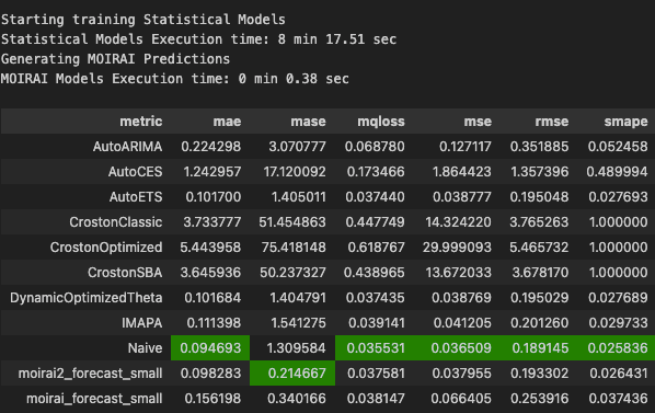
So, unfortunately, context length is not a data-determined parameter. It is a hyperparameter you have to tune.
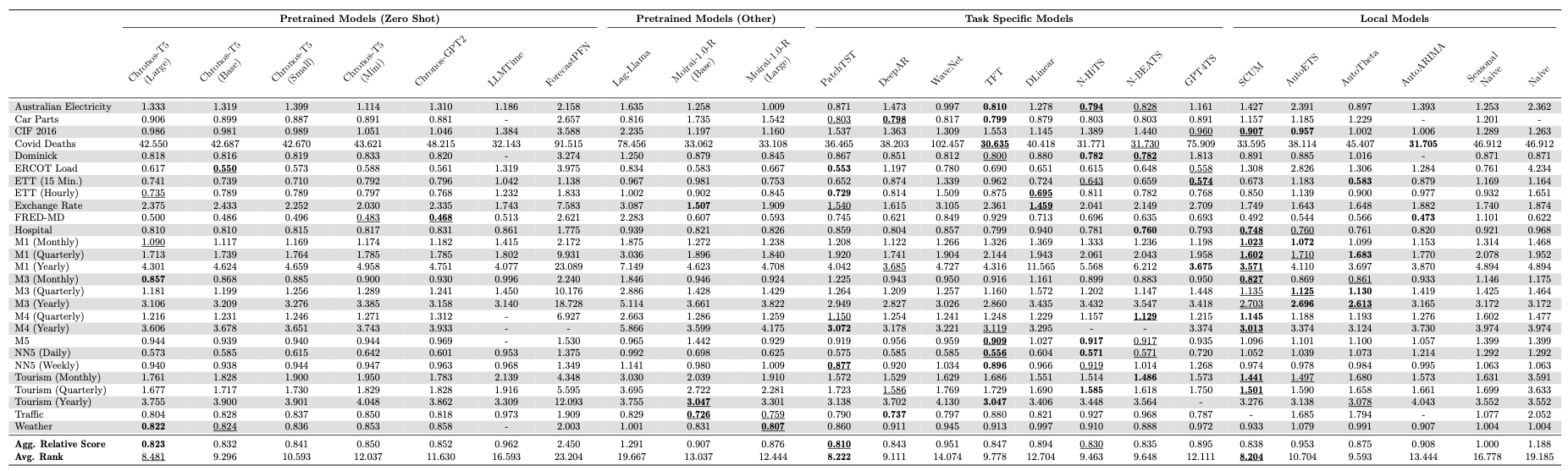
In the extreme cases where you have yearly, quarterly, or monthly data with very few datapoints, don’t bet that a foundation model will perform well, because the context length is not enough to capture any meaningful behavior. Keep in mind that foundation models are pretrained on much larger lengths
Prof. Christoph Bergmeir’s presentation at a NeurIPS’24 workshop [2] shared this image from Chronos, showing that SCUM (the famous Statistical ensemble of Fotios Petropoulos and Ivan Svetunkov[3]) outperforms Chronos-1 on Monash datasets where time series lengths are very small. For example, the M1 yearly dataset has as few as 15 datapoints and a forecasting horizon of 6!
How to address this:
Increasing context length often helps, but not always on tricky datasets. In those cases, run a train/validation split first and tune the context length instead of assuming the maximum value will win.
Yearly, quarterly, or monthly data with very short histories are especially challenging for TSFMs. In that regime, always compare against Naive, Seasonal Naive, and strong statistical baselines before trusting the foundation model output.
Scaling laws spearheaded the current LLM revolution — and given the multi-trillion-dollar bet of AI spending that relies on these laws leading us to AGI, they could also become the LLMs’ downfall.
Scaling Laws are empirical rules that describe the relationship between a model’s parameter size, tokens (dataset size), training time, and performance.
So the first instinct is to apply them to time series pretrained models. Initial experiments showed that increasing parameter counts and architecture complexity improved performance. There is additional research in this direction, confirming similar power-law trends [4] [5].
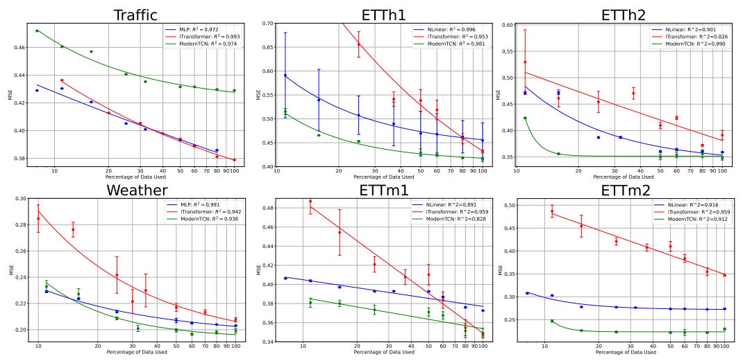
But the 2nd generation of foundation models scaled back this idea. They showed that beyond a point, adding parameters gives diminishing returns, while better pretraining techniques become more catalytic for performance.
Take Time-MoE as an example. It scales to 2.4B parameters, with ~1.1B activated due to mixture-of-experts routing. Despite this, larger size alone does not guarantee dominance over smaller, well-trained models. Also, Time-MoE-ultra has not been fully released at the time of writing this article.
In contrast, TimesFM-2.5 uses ~200M parameters (down from ~500M in TimesFM-2.0) and still improves performance.
What this means
Early TSFM papers show clear gains from scaling, but the pattern is not a clean copy of the LLM story: more data and more parameters help, yet bigger models do not always win. More research is needed on this.
Thus, time-series scaling laws are real, but they behave differently from the LLM case because model size, data size, and horizon choice all matter at the same time.
New research has shown that the key differentiator here is not scale alone, but the pretraining strategies. We’ll expand on this later in the article.
Almost all 1st-generation time series foundation models focused on univariate forecasting.
No issue with this — zero-shot forecasting itself was unproven at the time. The main goal was to show that TSFMs could beat classical supervised baselines. And on early benchmarks, they mostly did.
But in real-world projects, covariates are essential.
There are 4 main types:
Past observed (time-varying), e.g. air pressure
Future known (time-varying), e.g. day_of_week, is_holiday
Static categorical (time-invariant), e.g. product_color
Static numerical (time-invariant), e.g. initial account balance
And when it comes to forecasting, there are 4 modes:
Univariate forecasting (forecast each target time series independently)
Multivariate forecasting (forecast all target time series jointly, also known as channel-mixing)
Univariate Forecasting with Covariates (also called covariate-informed)
Multivariate Forecasting with Covariates (jointly forecast all target series, covariate-informed)
If these categories confuse you, check my Chronos-2 tutorial where I break them down with examples.
Among current models, the TTM family (Tiny-Time-Mixer) of models is the most versatile. Chronos-2 also supports multiple forecasting modes, although it has limitations with static variables (you can still use a global item_id in practice for grouped series like retail).
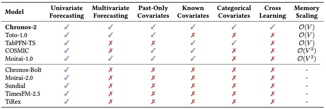
There is also the option to use an external regressor (TimesFM supports this). However, this excludes past observed inputs and defeats the zero-shot setup, since the regressor requires training. That trade-off may still be acceptable depending on the application.
What this means
In truth, foundation models have not yet fully explored multivariate forecasting. Only a handful of models tackle it properly, while most of the field still focuses on simplified setups and simply do univariate forecasting by assuming channel-independence, which is not applicable in complex, real-world datasets
Fortunately, newer versions are moving in that direction.
Chronos-2 and TTM already do a strong job of integrating covariates, making them practical for retail, financial, and energy forecasting.
But the real power lies ahead: combining multivariate structure with in-context learning and eventually multimodal forecasting.
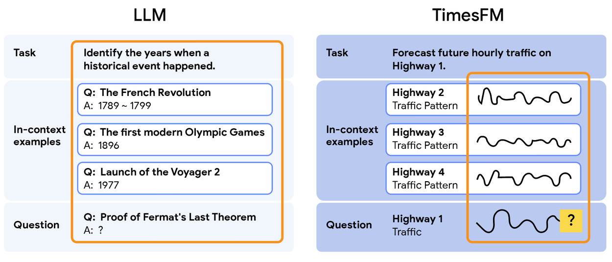
An interesting variant of TimesFM, called TimesFM-ICF, applies in-context learning elegantly. Unfortunately, it has not been released, and its architecture has not yet been widely explored by open-weight models.
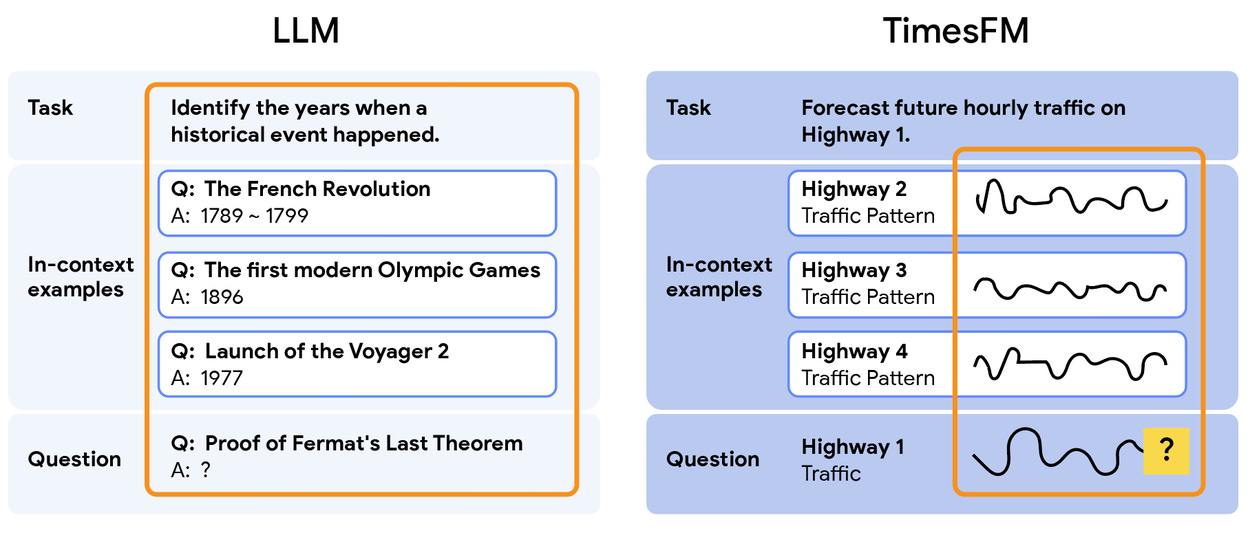
Figure 9: TimesFM-ICF example. Similar to few-shot prompting of an LLM (left), a time-series foundation model should support few-shot prompting with an arbitrary number of related in-context time series examples (right). The orange box encloses the inputs to the models. (Source 6) The endgame for time series foundation models is multimodal forecasting. A recent example is Migas-1.5, which combines text and time series in a unified framework [7]. We’ll explore this model in a future article.
While interpretability seems straightforward for simpler statistical models, that’s not the case for neural-based or Transformer-based models. Of course, every time series foundation model is neural-based.
There are 3 main ways to explain predictions from a neural-based model:
Model-agnostic methods: Perturbation-based approaches such as SHAP.
Built-in methods: For example, learned feature gates or attention-style modules that expose importances, similar to what happens in TFT and TTM
Layer/gradient attribution methods: These still use the internal knowledge of the model, but are more generalizable. e.g., Captum’s integrated gradient method. Last month, NeuralForecast made a significant breakthrough by providing interpretability using Captum for DL-based models.
It is commonly assumed that foundation models are not interpretable either. However, TimeGPT provides interpretability through SHAP. The way it is probably done is by computing SHAP on exogenous covariates, like future holidays, weather, or price, which can be shuffled more naturally alongside the target series. TimeGPT also provides feature importances across prediction steps, which is extremely useful. Still, TimeGPT is a closed model, and the exact method is unknown.
Time series SHAP is trickier than tabular SHAP, because you cannot always “turn off” one historical timestep (e.g., t−5) without breaking the sequence structure. There are also surrogate methods, such as TsSHAP, that build explanations from user-defined features and then explain a black-box forecaster through a surrogate model.
Interpretability in time series foundation models is totally feasible, but it hasn’t been explored in depth yet. Glancing through the recent ICLR Workshop on Time Series in the Age of Large Models [8], I see several interesting implementations that I’ll cover in a future article. One of them [9] applies a sparse autoencoder on Chronos-2’s hidden states to assess feature reconstruction, which leads to feature-level interpretability.
This is my favourite topic.
When I scroll through LinkedIn, I will likely find a post about time series foundation models and the issue of data leakage.
Usually, it goes something like this: model X performed better because that dataset might be included in the model’s pretraining dataset, or it might be similar to a dataset included in the pretraining dataset, or we simply cannot trust that the dataset was not included — even though all time series foundation model papers disclose their pretrain/test splits (except if they are privated/copyrighted datasets).
We now also have leakage-resistant benchmarks like TS-Arena [10], where predictions are made on unseen data via pre-registration, so data leakage simply cannot happen there.
In truth, this discussion is pointless because the largest impact when training time series foundation models is synthetic data, emphasizing the pretraining techniques. This is more apparent in the Chronos-2 paper, where Chronos-2 barely surpasses the Chronos-2-synth model (trained purely on synthetic data).
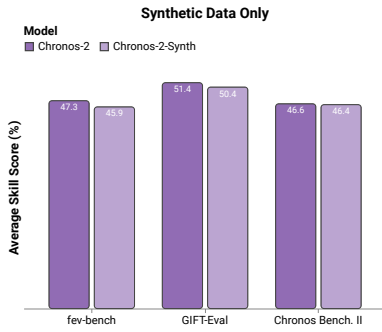
In fact, the pretraining techniques and synthetic data generator models are so successful that they are reused across models. For example, KernelSynth, introduced in Chronos-1, was also used in MOIRAI-2.
Recent implementations also focus on advanced, high-quality temporal synthetic data generators. For instance, [11] uses an optimized SARIMA data generator, producing zero-shot models that surpass their counterparts trained on real-world data as well.
Finally, we have all witnessed the revolution of tabular foundation models and the battle of PFN-based models. TabICL and TabPFN, which continuously surpass one another on TabArena, are trained purely on synthetic data and leveraging powerful prior data generator engines.
Time series is a different modality, but it might be the case that real-world temporal data will not be needed to train a TSFM. In any case, the aforementioned models (TabICL and TabPFN) have already taken steps toward time series — like TabICLv2 that we saw in our earlier article. We’ll see!
Time series foundation models are a major step forward, but they are not the final answer yet.
They work well in some settings, struggle in others, and still depend on the right data, the right context, and the right expectations. The main lesson is simple: use them where they are strong, tune them or use the right workarounds where they are fragile, and do not confuse convenience with universal power - because it doesn’t exist in time series.
Horizon AI Forecast is a reader-supported newsletter, featuring occasional bonus posts for supporters. Your support through a paid subscription would be greatly appreciated.
[1] Yu et al. Understanding the Implicit Biases of Design Choices for Time Series Foundation Models
[2] Bergmeir Christoph. Fundamental limitations of foundational forecasting models: The need for multimodality and rigorous evaluation
[3] Petropoulos and Svetunkov. A simple combination of univariate models
[4] Edwards et al. Scaling-laws for Large Time-series Models
[5] Shi et al. Scaling Law for Time Series Forecasting
[6] Sen and Zhou. Time series foundation models can be few-shot learners
[7] Synthefy (2026). Migas-1.5: Text-Conditioned Time Series Forecasting.
[8] Time Series in the Age of Large Models workshop.
[9] Divo et al. Finding the Zeitgeist in Time Series Foundation Models
[10] Meyer et al. TS-Arena: A Live Forecast Pre-Registration Platform for Leakage-Free Evaluation of Time Series Foundation Models
[11] Oreshkin et al. Zero-shot Forecasting by Simulation Alone
[12] Ansari et al. Chronos-2: From Univariate to Universal Forecasting
[13] Cohen et al. Toto and BOOM unleashed: Datadog releases a state-of-the-art open-weights time series foundation model and an observability benchmark
[14] Woo et al. Unified Training of Universal Time Series Forecasting Transformers (February 2024)
[15] Liu et al. Moirai 2.0: When Less Is More for Time Series Forecasting (November 2025)
[16] Google Research. TimesFM
[17] Ansari et al. Chronos: Learning the Language of Time Series
[18] Ekambaram et al., Tiny Time Mixers (TTMs): Fast Pre-trained Models for Enhanced Zero/Few-Shot Forecasting of Multivariate Time Series (April 2024)
Comments
Nothing yet. Say the first thing.
Sign in to join the conversation.