Adapting Time-Series Foundation Models at Inference Time

Google Research’s new paper is a significant milestone in the time series field

It’s well established that zero-forecasting works - however, in some datasets, a fully-tuned model can outperform a zero-shot model. This makes sense. How can a general model, however powerful on a benchmark, optimally capture the nuances of a dataset?

We can also fine-tune the pretrained model and further enhance its performance. But that defeats the purpose of zero-shot forecasting!

What if the model could adapt itself at inference time — without retraining, gradient updates, or losing its generality? That’s exactly what this paper explores!

The authors propose a foundation model (based on TimesFM) that can learn from context. At inference, it takes multiple related time-series as examples — alongside the target’s own history — and uses them to adjust its forecasts. The model behaves as if fine-tuned on the fly, guided only by the data it sees in context.

The results are striking. This in-context adaptation not only improves performance on standard benchmarks but can also match the accuracy of a model that has been explicitly fine-tuned on the target domain.

Let’s get started!

✅ Find a tutorial notebook on TimesFM, along with other cool projects here: AI Projects Folder (Project 24)

The authors use this term throughout the paper, but simply put:

In-Context Fine-Tuning bridges the gap between zero-shot and fine-tuned forecasting - making a foundation model perform as it’s fine-tuned on the whole dataset

In LLM terms, it’s like adding extra info to a prompt, guiding the model toward a more informed response. This is called “in-context learning” in NLP, and it’s known since GPT-2. See Figure 1 for an example:

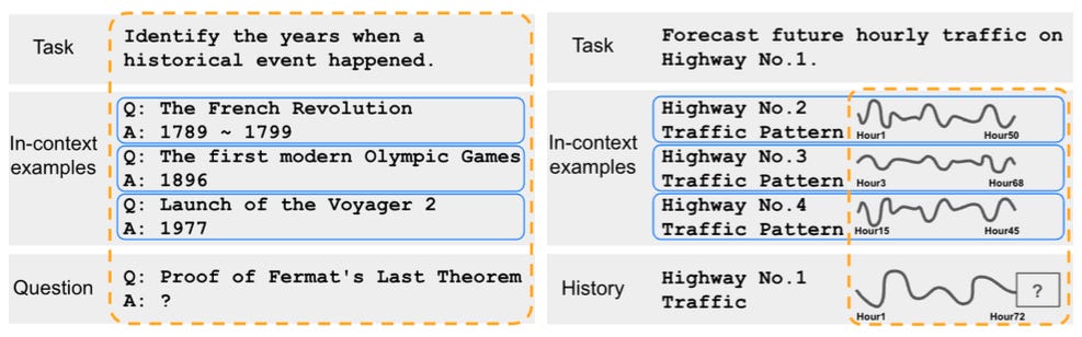
But applying this to a general pretrained time-series model isn’t easy. Each input must be temporally aligned. How can a model tell what’s past data versus what’s context examples—especially when those examples are unordered or discontinuous?

The authors test their approach on TimesFM, though it can work for any decoder-only univariate foundation model. The main contributions of the paper are:

• In-context fine-tuning: Introduces a new way for time-series foundation models to adapt at inference time using context examples — related series placed alongside the target history in the prompt.

• Training methodology: Extends a pretrained decoder-only model through continued pretraining with variable-length histories, horizons, and multiple in-context examples — enabling it to “borrow” temporal patterns from related series.

• Adaptive forecasting: Shows that the model learns to adapt to new domains on the fly, leveraging contextual signals rather than explicit retraining or gradient updates.

• Empirical gains: Demonstrates strong performance across 23 unseen datasets, improving zero-shot accuracy by 6.8% over the base model and 5% over the best existing baselines.

• Fine-tuning equivalence: Achieves performance on par with models explicitly fine-tuned on each dataset — proving that context alone can drive adaptation.

Note: Have you heard of distilling reasoning models such as Qwen-Distilled-R1?

These models take non-reasoning base models (like Qwen) and fine-tune them on reasoning text messages generated by larger reasoning models. The training data often include tags like <think> and </think> to mark internal thought sequences, encouraging the model to produce self-correcting reasoning steps. We do something similar here, except our context involves time-series examples.

And if you’re thinking that reasoning in LLMs still boils down to next-word prediction, you’re absolutely right!

Here, the authors start with the base TimesFM model, introduce key adaptations (creating TimesFM-ICF), and adjust the pretraining dataset to enhance the new model. Let’s see how they did it in the next sections.

As mentioned earlier, adding time series data as model context is challenging.

Unlike language models, we can’t just append time steps like words. Doing so changes the series’ dynamics (see Figure 2).

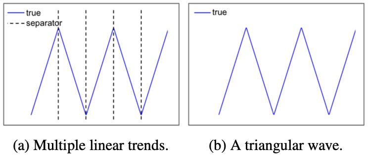
You might ask: Why not use a multivariate model and add the context as extra variables? In fact, MOIRAI-1 is a native multivariate model.

Well, a multivariate model expects the additional features to be temporarily aligned with the target variable and directly affecting it (Granger causality). But our goal here is to transfer contextual signals, not model feature dependencies.

Moreover, building a multivariate foundation model that generalizes across datasets is impractical. How could it infer every possible interdependency so well that it can generalize well to an unseen dataset? That’s why MOIRAI-2 dropped multivariate support and became a univariate, decoder-only model. (as we explained here).

Hence, enabling a univariate model to adapt during inference with external context makes more sense!

Let’s now examine the proposed methodology.

The authors begin with the original TimesFM model, pretrained as described in an earlier article. The input is defined as a univariate time series with lookback length L and forecast horizon H.

In TimesFM-ICF, the input changes: besides the target series history L, the model also receives n = 50 context examples of related time series. Each example has a maximum length T = L + H, with variable lengths padded if needed.

To avoid the confusion of Figure 2, the authors introduce a trainable separator token to separate the context examples (Figure 3).

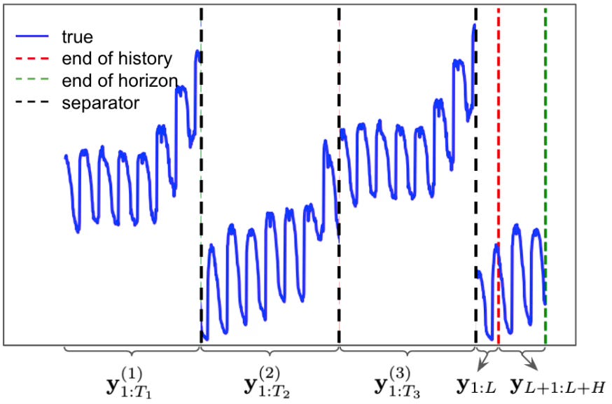
Hence, the separator token is just a shared learnt embedding vector - inserted after each context example.

As in the original TimesFM, TimesFM-ICF splits both input and output into patches, where len(input_patch)=32 and len(output_patch)=128.

For each training example i in [1, 50], the series is divided into p patches. Each patch is tokenized and fed sequentially/autoregressively into the model, followed by the separator token (Figure 4).

Note: Feel free to read my article on TimesFM-1 to get a refresher! TimesFM-ICF uses the same components as TimesFM-1 (the “base TimesFM” as the authors call it). Don’t confuse TimesFM-2.5 with TimesFM-ICF — TimesFM-2.5 is just a more advanced checkpoint of TimesFM-1, but without in-context forecasting.

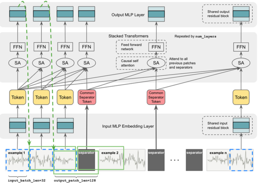
To help the model distinguish different in-context examples, the authors let the transformer causally attend to all previous patches, including the separator tokens. This is essential — without attending to these tokens, the model couldn’t distinguish between example boundaries, as shown in Figures 4a and 4b.

By attending to separators, the model learns how many in-context examples have been processed and where each one starts and ends. This mechanism gives the transformer a clear sense of structure across multiple examples.

While the separator token begins as a simple shared embedding, it takes on a richer role through the layers. The output tokens of the separator tokens gradually summarize their examples’ patches and signal the boundaries between examples, helping TimesFM-ICF learn more structured and meaningful temporal relationships.

Note: The model is pretrained not only on the target series but also on the context examples. It randomly masks datapoints in the first patch so the model doesn’t overfit to context lengths that are multiples of the input patch size.

That’s why the authors supply an extra binary padding mask vector with the input (1 = masked datapoint). If an entire patch is masked, attention is not applied to it. For more details, see the original paper.

Now, 2 main questions arise:

1. Given a training time series, how do we find relevant example time series in the rest of the dataset?

2. What is the final pretraining format for TimesFM-ICF?

Relevant Context Examples
The authors tested several methods, including complex ones such as DTW, to find the 20% most similar time series.

Eventually, after ablation studies, they chose a simpler setup: n = 50 context examples—5 from the target series’ recent history and 45 randomly sampled from other series in the same dataset.

Final Pretraining Format
The authors use a portion of base TimesFM’s pretraining dataset to generate context examples.

Recall that the TimesFM base model is trained with a maximum history length of Lmax = 512, and during training, a time-series of length T = Lmax + h = 640 (with h = 128 as the output patch) is used for backpropagation (like I explained earlier).

Therefore, in TimesFM-ICF, T becomes the maximum length for each in-context example. Using a windowing stride of 1, the authors generate overlapping segments of length T from each time series, padding shorter ones as needed to preserve consistency.

To form the context, these examples are grouped in 2 ways:

• Time-series level: split one long sequence into multiple T-length segments, selecting n to form the context.

• Dataset level: sample n segments from different series within the same dataset for greater diversity.

Let’s say during training we have loaded a time series from the Electricity dataset (which has 370 time series in total, hence belonging to dataset-level grouping). We can use any n=50 time series from the Electricity dataset to form the context - allowing the model to capture correlated temporal patterns across related signals.

Adding context examples increases complexity.

Thus, the paper examines the trade-off between performance and inference time as context size grows. The results are shown in Figure 5:

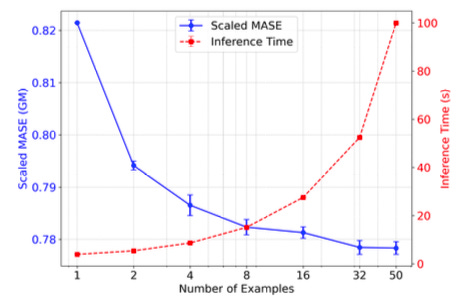
Indeed, as we add more in-context examples, the error steadily drops—but this comes at a cost: inference takes longer, revealing a clear trade-off.

One of the longest-standing myths in forecasting is that Transformers are unsuitable for time series because self-attention is permutation-invariant.

Since attention is computed as pairwise scores between observations, changing their order does not affect these scores —which is true and problematic for sequential data.

However, this claim has been misused. Since 2020, nearly all major Transformer-based forecasting models leverage positional information through explicit encodings or attention applied between features, where order invariance is irrelevant.

In this work, the authors take a bold step further: they remove positional embeddings entirely (NoPE, meaning No Positional Encoding). Surprisingly, their experiments show that the model performs on par with those using positional embeddings:

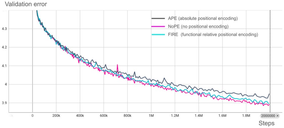
This happens for 2 main reasons (the first noted in the paper):

• Causal attention (unlike standard self-attention) implicitly encodes positional information once a single Transformer layer is present. This effect compounds in a well-pretrained, generalizable model.

• MLPs within each Transformer block inherently capture positional patterns. That’s why linear DL models like TSMixer are also successful.

Fortunately, NoPE setup brings key advantages during continued pretraining:

• Better length generalization — crucial when extending context windows with in-context examples, as NoPE models handle longer prompts more gracefully.

• Semantic consistency — removing absolute encodings avoids mismatch between base model training (without examples) and continued pretraining (with added context), preventing positional drift.

• No accuracy trade-off — empirically, NoPE maintains validation performance comparable to advanced length-generalizing encodings like FIRE.

Hence, we can now use TimesFM with variable context and prediction lengths!

Also, let’s hope this article helps clear up the misconceptions about permutation-invariant attention.

The authors evaluate TimesFM-ICF (In-Context Fine-tuned) on the Chronos Zero-Shot Benchmark (OOD) — a diverse collection of 27 datasets spanning multiple domains (finance, demand, weather, traffic) and granularities (minutes to years). None of these datasets, including their training splits, were used during pretraining.

Let’s describe the setup:

• Goal: Test whether TimesFM-ICF can match the fine-tuned baseline (TimesFM-FT) without gradient updates during inference.

• Metric: Normalized MASE, scaled by a seasonal naive baseline; performance aggregated using the Geometric Mean.

The results are shown in Figure 7:

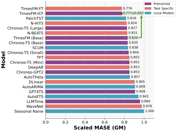
• TimesFM-FT remains the strongest overall, as expected from its dataset-specific fine-tuning.

• TimesFM-ICF, however, matches TimesFM-FT’s performance zero-shot, using only in-context examples!

• Gains of +6.8% over the base TimesFM model and +5% over the next best non-TimesFM baseline (PatchTST).

• Despite higher per-forecast cost, TimesFM-ICF completes the full OOD benchmark 16× faster (25 min vs 418 min).

The authors also implement a few other benchmarks - feel free to read the original paper for extra info!

TimesFM-ICF marks a milestone for time-series foundation models.

Specifically, TimesFM-ICF demonstrates true in-context adaptation — achieving fine-tuned-level accuracy with no retraining. This positions it as a practical, zero-shot alternative to conventional fine-tuning for supervised learning

Of course, there’s still room to improve, such as refining how examples are selected or reducing inference time.

Most importantly, this method can be applied to any decoder-only attention-based foundation forecasting model!

Horizon AI Forecast is a reader-supported newsletter, featuring occasional bonus posts for supporters. Your support through a paid subscription would be greatly appreciated.

1. Das et al. In-context Fine-tuning for Time-series Foundation Models (ICML 2025) - All images here are from the current paper