What Makes a Kernel Learnable

Chapter 7 of The Learned Kernel. The previous chapters argued that the geometry, the kernel, should be learned rather than chosen. Learning the geometry introduces a failure mode that a fixed kernel does not have: the model can overfit the geometry itself and then report a score it cannot reproduce on new data. This chapter is about detecting that failure, and the remedy is a single held-out fold.

Consider the following measurement. The gradient-boosted tree ensemble from Chapter 4, shown there to be a kernel machine with a learned leaf similarity, is fit on a set of California housing blocks and then asked to predict those same blocks. It scores an R² of 1.00. The residuals are essentially zero.

A second set of blocks, which the ensemble never saw, is then held out and predicted. The R² falls to 0.72.

The kernel and the model are identical in both cases. The first number reports a flawless fit and the second reports a good but unremarkable one. A selection procedure that looked only at the first number would prefer this kernel every time, and for the wrong reason. The 1.00 does not reflect an understanding of the data. It reflects memorization of it.

The gap between how good a learned kernel appears on its own training data and how good it is on new data is the subject of this chapter. It has a specific cause, a simple remedy and a piece of theory that turns the remedy into a design principle.

Every kernel method in this series makes its prediction by smoothing. Each can be written as

where x is the vector of observed targets and S is the smoother matrix that combines them into predictions. A simple averaging kernel produces a gentle S that mixes each point with its neighbors. A flexible kernel produces an aggressive S that can route almost all of a point’s prediction onto the point itself.

The quantity of interest is whether ŷ is close to the truth, meaning the clean signal beneath the noisy labels. Call that the risk. The quantity that is actually observable is the in-sample residual, meaning how far the predictions fall from the noisy training labels. These are not the same, and the difference is the central point. For mean-zero noise of variance σ² they are related by an exact identity:

Read the identity from left to right. The observable in-sample residual on the left equals the risk, plus the noise floor σ², minus a correction term built from tr S, the trace of the smoother, which counts its effective degrees of freedom.

The consequence is the key point. A flexible, near-interpolating kernel drives tr S toward its maximum. As it does, the correction term grows and the observed in-sample residual falls below the noise floor σ². The model then appears to have removed more error than the noise contains, which is impossible and is a direct signature of memorization.

Any selection rule that rewards a small in-sample residual is therefore biased. It does not reward the kernel that best explains the data. It rewards the kernel that can bend most to fit it. The most flexible geometry wins every in-sample comparison because it can conceal its errors inside the fit. This is the over-credit problem.

The remedy is simple and it is the same discipline used for the out-of-fold residuals in Chapter 4. Split the rows into two sets:

• a support set, used to build each candidate kernel (fit the ensemble, fit the length scales, set the bandwidth), and

• a query set, held out and used only to score the kernel.

A kernel then receives credit only for predicting points it never saw. The supervised ensemble built its leaf partition on the support set, so predicting the query set no longer lets it route the answer onto a memorized neighbor. It has to generalize, and its score reflects whether it can.

Concretely, build the support-to-support kernel block K_SS and the query-to-support block K_QS, solve for the prediction weights on the support and measure the error on the query fold:

The prediction K_QS is scored against the held-out query labels, and the support set is never graded on itself. This procedure, fit on support and score on query, underlies the remainder of the book. The spectral kernel of the next chapter is fit this way. The fusion of several kernels is selected this way. The in-context method at the end of the book, which learns a kernel from examples, is the same split amortized across many tasks.

Consider three candidate kernels on California, each fit on the support fold:

• a plain RBF kernel with a bandwidth chosen by the modeler,

• the ARD kernel from Chapter 3 with per-feature length scales that are learned, and

• the supervised leaf kernel from Chapter 4.

Each kernel is scored alone, in-sample and on the query fold:

Consider the gap column. The RBF and ARD kernels have modest gaps of 0.16 and 0.12 between their support and query R². They do not fit their training data perfectly, so they overstate their quality only slightly. The leaf kernel is different, with a support R² of 1.00, a query R² of 0.72 and a gap of 0.28. Its in-sample score roughly doubles its true performance. This is the channel on which the leakage-free selector and the in-sample selector disagree most.

The three kernels are then combined into a single fused kernel, a weighted mixture, and two rules select the weights. The first scores the mixture in-sample, using a classical criterion called SURE that is discussed below. The second scores it on the held-out query fold.

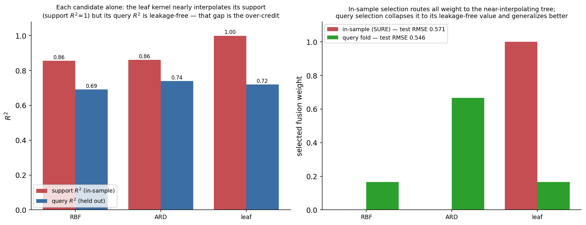
The left panel shows the same ledger as bars, with the leaf kernel’s support bar at 1.00 and its query bar at 0.72. The right panel shows the consequence. The in-sample rule assigns all the weight to the leaf kernel, with RBF 0.00, ARD 0.00 and leaf 1.00, and sets the regularization to nearly zero. It also estimates the noise variance at σ² ≈ 0.002, which effectively declares the data noiseless, because the memorizing kernel has accounted for every fluctuation.

The query rule does not:

It reduces the leaf kernel’s weight from 1.00 to 0.17 and assigns the majority of the mixture, 0.67, to the learned ARD geometry, which was the best generalizer of the three at a query R² of 0.74. The result is a lower error: the query-selected mixture scores a test RMSE of 0.546 against 0.571 for the in-sample mixture. The leakage-free rule selected the model that predicts better on unseen data.

The effect is larger on the Taiwan credit-default data. There the leaf kernel posts a support R² of 0.999 and a query R² of 0.013. A deep ensemble can memorize the binary default labels almost perfectly while carrying essentially nothing to new customers. In-sample the fit appears excellent. On the query fold it is barely better than chance.

SURE, Stein’s Unbiased Risk Estimate, was mentioned above. It is a sound method applied in the wrong place rather than a poor one.

SURE inverts the identity given earlier. If the in-sample residual is too small by exactly (2σ²/p)·tr S − σ², that quantity is added back:

For a kernel fixed in advance, chosen before the labels were examined, this correction is exact. SURE is a provably unbiased estimate of the true risk, requiring only that the noise has mean zero and variance σ², with no assumption of normality. The proof is in the book.

Its behavior can be checked on a controlled problem where the truth is known. Construct a synthetic signal f, add noise and denoise it with a fixed kernel while sweeping the regularization λ. Because f is known, the true risk can be computed and compared against SURE.

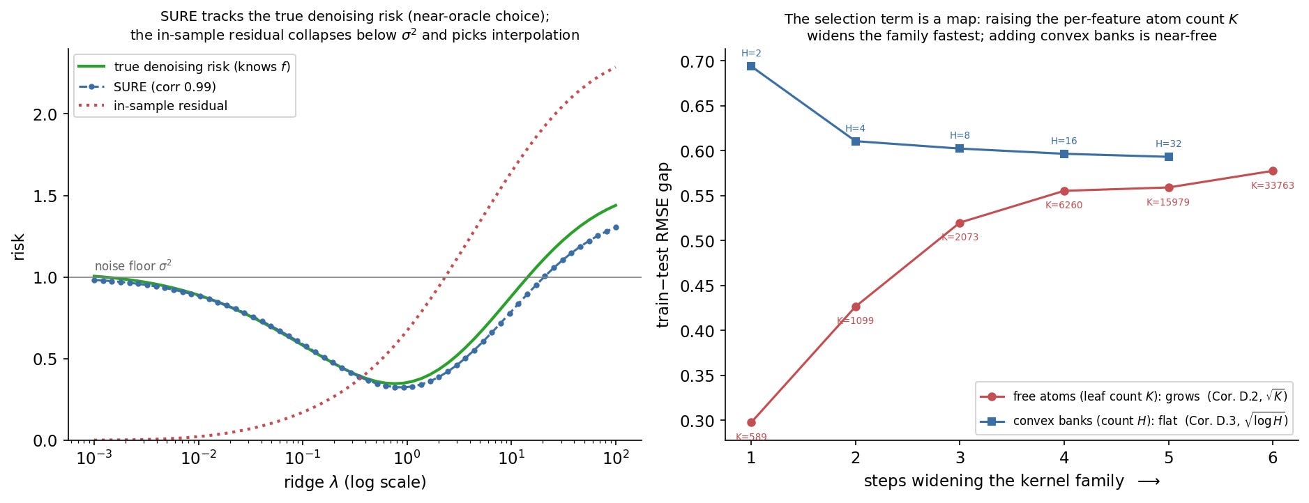
In the left panel the green curve is the true risk and the blue dashed curve is SURE. They track each other at a correlation of 0.99, and the λ chosen by SURE gives a true risk of 0.350 against an oracle best of 0.347. The red dotted curve is the raw in-sample residual. It falls to zero as λ shrinks, drops below the noise floor σ² and would select λ = 0, pure interpolation, whose true risk is three times the oracle. SURE corrects precisely the optimism that the raw residual exhibits.

Why then did SURE fail on the leaf kernel above? SURE’s guarantee carries a condition: the smoother must be fixed with respect to the noise it is denoising. A chosen RBF satisfies this. An ensemble fit to the same labels it then denoises does not, because its S depends on the noise; boosting fit the splits to that noise. SURE’s trace correction cannot see the degrees of freedom the ensemble spent searching for its partition, so it undercounts the leaf kernel’s flexibility and over-credits it. The remedy is the split used above: build the kernel on the support fold so that it is fixed relative to the query fold’s noise. SURE, or more simply the query R², is then leakage-free.

The rule is general. If the kernel’s construction used the labels it is scored on, an in-sample criterion will overstate its quality. Hold out a fold.

There is a piece of theory beneath this whose shape, even without the proof, is the practical lesson. When a kernel is learned from a family of options and then used to predict, the error decomposes into two terms:

The first term is the cost every kernel machine pays to fit a predictor once the kernel is fixed. The second is the additional cost of having chosen the kernel, and its size is set by 𝔠(Θ), the number of free parameters in the kernel family. The more parameters the geometry has, the more ways it can chase noise and the larger this selection cost. The query fold is the instrument that keeps the second term leakage-free.

This cost is not a single quantity. It itemizes, and the itemization shows which design choices are expensive and which are nearly free. The right panel of the figure above shows two of them on California.

The red line is the expensive axis. As the leaf kernel is given more raw atoms, meaning deeper trees and more leaves, here from 589 to 33,763, the gap between training and test error rises steadily from 0.30 to 0.58. Each additional free atom is another opportunity to overfit. This is the variance to control.

The blue line is the cheap axis. As more bandwidth banks are combined in a convex mixture, from 2 to 32 scales, the gap barely moves; it drifts down slightly and then flattens near 0.60. The theory explains this: banks enter through a convex mixture, and the cost of a convex mixture grows like the logarithm of the number of banks rather than the number itself. Adding multi-scale richness is therefore nearly free, while adding raw atoms is not.

This distinction, that one parameter costs variance while another is nearly free, is the design principle behind the spectral chapter and the fusion chapter. Capacity is spent where it buys structure and withheld where it buys only memorization.

A third option on the map makes the next chapter possible. Instead of giving the kernel a long list of free frequencies to set individually, the expensive red axis, one describes those frequencies with a short density, a few numbers that specify where the energy is concentrated and how spread out it is. The number of frequencies can then be raised as high as needed to resolve a sharp pattern without changing the cost, because only the few density parameters are learned rather than the frequencies themselves. Capacity is decoupled from resolution. This is how the spectral kernel of the next chapter can be both sharp and safe: it learns a smooth spectral density rather than a set of free atoms and scores that density on the held-out query fold, the same leakage-free fold used throughout.

None of this depends on the constants in the bound, which is an upper limit and a loose one. What it provides is the shape of the problem: a fixed cost for fitting plus a selection cost determined by how the geometry is parameterized. The engineering follows from that shape. Use few well-structured parameters, combine kernels through convex mixtures rather than free-fitting and do not read the selection cost off the training fold.

The leakage-free and in-sample selectors differ by one line, the fold on which the score is computed:

for w in simplex_grid(C, res):                 # candidate blend weights
    Kss = mix(Bss, w); Kqs = mix(Bqs, w)
    th, V = np.linalg.eigh(Kss)                # eigendecompose once
    Vtyc = V.T @ (ys - ybar); M = Kqs @ V
    for lam in lam_grid:
        coef = Vtyc / (th + lam)
        r2_query = r2(M @ coef + ybar, yq)     # HELD-OUT query: leakage-free
        df  = np.sum(th / (th + lam))
        rss = np.sum((lam / (th + lam))**2 * (Vtyc**2))
        sure = rss/n + 2*sigma2*df/n - sigma2  # IN-SAMPLE: leaks for a learned kernel

Selecting the (w, λ) with the best r2_query gives the leakage-free mixture; selecting the best sure gives the over-credited leaf kernel. The companion notebook builds all three kernels, reproduces the ledger and the selection contrast, runs the SURE-tracking experiment and provides a slider for watching the in-sample residual mislead while SURE and the true risk agree.

▶ Run it in Colab (no install): open in Colab

📦 Code: github.com/asudjianto-xml/Learned-Kernel

The previous installment, Every Prediction Carries Its Own Evidence, introduces the smoothing view of the prediction; the S matrix in this post is that weighted vote written as a matrix.

A learned kernel is more powerful than a chosen one, and the added power carries a risk. A kernel flexible enough to learn the geometry is flexible enough to memorize the noise, and its in-sample score will not distinguish the two. The reliable way to tell them apart is to score the kernel on data it has not seen. Hold out a query fold, score the kernel there and report the gap between its training-data claim and its held-out performance. That gap is the credit the kernel has not earned. The next chapter builds the geometry directly in the frequency domain: the spectral kernel.

The Learned Kernel is a free weekly series adapted from my book of the same name. The posts carry the intuition and the runnable code; the book carries the full derivations, including the proof that SURE is exactly unbiased and the two-term bound behind the capacity map.