Trees Knew Where the Model Was Weak. Now a Mixture of Experts Repairs It.

Post 5 of The Learned Kernel. Last time we showed that a gradient-boosted ensemble carries its own map of where it fails — read the leaf kernel, cluster by it, and the weak regions surface on their own. I promised we’d act on that map. This is the repair — and we do it in credit, where the fix is only allowed if it keeps the model monotone and readable.

Last chapter we made a black box do something it is not supposed to allow: tell us where it was weak (https://agussudjianto.substack.com/p/trees-are-kernels-and-the-kernel). A gradient-boosted tree ensemble on California housing looked like a solid, shippable 0.85 R² — until we read its own leaf kernel, clustered the data by the geometry the model actually uses, and watched that average shatter into pockets, one of them far worse than the rest. The kernel drew the map. Then I made a promise: next we would repair the weak region without disturbing the parts that already work.

This is that chapter. But we are going to change the setting on purpose — because repair is easy when nothing is at stake, and the whole point is what happens when something is.

Repair is trivial if you are free to do anything: bolt on capacity, drop in a local model, let it fit whatever it likes in the weak pocket. It gets interesting — and actually useful — when you are not free. In credit, the same model that locates the weak region has to stay monotone and explainable, because someone will be declined by it and someone else will audit that decision. So we move from housing to lending, where “fix the weak spot” only counts if the fix breaks none of the guarantees that let you ship the model at all. That constraint is the entire game.

So you are building a credit default model, and the tension shows up before you write a line of it.

You can train an unconstrained gradient-boosted ensemble. On our data — ten thousand applicants, ten risk drivers, a default flag — a depth-2 CatBoost does that at an out-of-sample AUC of about 0.92. It is accurate. It is also un-shippable, and you know it the moment you try to explain a declined application to the person who was declined, or to the regulator who asks you to.

Or you can build a model you can defend: monotone in every driver, readable end to end. Constrain that same CatBoost and the AUC falls to about 0.81.

That drop — 0.92 down to 0.81 — is the tax on trust. This chapter is about getting most of it back without paying it back in trust, and the instrument, again, is the kernel the model grows for free.

Why does the constrained model give up a tenth of an AUC? Look at what the free model was doing to earn it.

Because we cap the trees at depth two, the ensemble is not an opaque stack. That one setting is doing more work than it looks, so it is worth unpacking.

Any function of several variables can be written as a sum of pieces of increasing order — a constant, one term per feature, one term per pair, and so on:

That is the functional ANOVA decomposition (https://modeva.ai/docs/2-user-guide/models/gbdt#interpretability-through-functional-anova). The constant is the global level, f_j is what feature j does on its own — its main effect — and f_jk is what the pair does that neither does alone. The decomposition is completely general. The trouble, for a typical model, is that the series runs to high order and the individual terms are not separately meaningful.

Tree depth truncates it exactly. A tree of depth d routes a point through at most d splits, so any leaf involves at most d distinct features — the ensemble cannot express an interaction of higher order than d. Depth 1 leaves you main effects alone: a GAM. Depth 2 leaves main effects plus pairwise interactions and nothing beyond: a GAM with interactions. This is a structural fact about the model, not an approximation of it.

Reading the terms off takes two stages. First aggregation: sort every leaf in every tree by how many distinct features appear on its path — one feature makes it a main effect, two make it a pairwise interaction — and sum the leaf values into the matching term. Second purification: the raw aggregated terms are not identifiable, because a main effect can hide inside a pairwise term that contains it, and several different bookkeepings give the same predictions. Purification sweeps the means out of the interactions into the main effects, iterating until every term is zero-mean and all terms are mutually orthogonal. Only after that does “the effect of utilization“ name one specific thing.

The payoff is that the shapes below are the model — not a surrogate fitted afterwards to imitate it, and not a post-hoc attribution. Modeva reads the decomposition straight out of the fitted CatBoost. (The construction is in Inherently Interpretable Tree Ensemble Learning.)

So read the free model’s effect for utilization — the share of available credit an applicant is using:

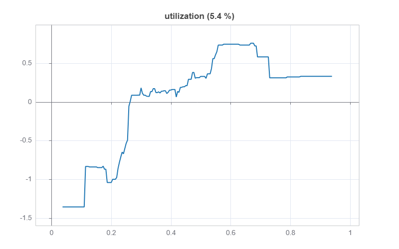
It wiggles. It rises, then dips, then rises again. In stretches, higher utilization makes the model predict less default risk. That is not a signal anyone believes; it is the model contorting itself to fit noise in the training sample, and it is a good part of where that extra AUC came from. A credit analyst would reject the shape on sight. A regulator would fail it.

Now the same effect in the monotone model:

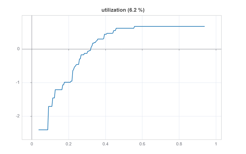
Clean, and strictly increasing. More utilization, more risk, everywhere — a shape you can put your name on. That is the trade the accuracy table just priced for us: a little discrimination surrendered in exchange for a model that refuses to fit nonsense. Effect importance confirms the model is dominated by a few clean drivers — score far and away first, then tenure and dti — with the interaction terms small. It is almost additive, which is exactly what makes it readable.

The constrained model is honest. It is also, at 0.81, leaving accuracy on the table. The question is whether 0.81 is really the best an honest model can do — and the answer is no.

This is the thread from Chapter 4, and the mechanism is identical — only the model has changed. There the kernel came from an XGBoost on housing; here it comes from our monotone CatBoost on credit. A tree ensemble splits the space into leaves; two applicants are similar, in the model’s own eyes, when they fall in the same leaves across the trees. That leaf co-membership is a genuine kernel K, and it is supervised — it measures closeness the way the model actually reasons about default, not the way raw features happen to line up.

In Modeva you obtain exactly that kernel by restricting a FuseKernel to its tree channel — no RBF, no learned spectral component — and pointing it at the same tuned, monotone CatBoost:

gbdt_params = {**best_params, "depth": 2, "monotone_constraints": mono}
fk = MoFuseKernelClassifier(backend="catboost",
                            use_xgb=True, use_rbf=False, use_spectral=False,
                            solver="nystrom", gbdt_params=gbdt_params)
fk.fit(ds.train_x, ds.train_y.ravel())

We will not predict with this kernel. We will navigate by it.

diagnose_weak_clusters (https://modeva.ai/docs/2-user-guide/testing/fusekernel_repair) builds a degree-normalized Nyström spectral embedding of K — landmarks keep the eigensolve linear in the sample size — clusters the applicants in that embedding, and scores the model cluster by cluster.

weak = fk.diagnose_weak_clusters(ds, n_clusters=5)
weak.plot()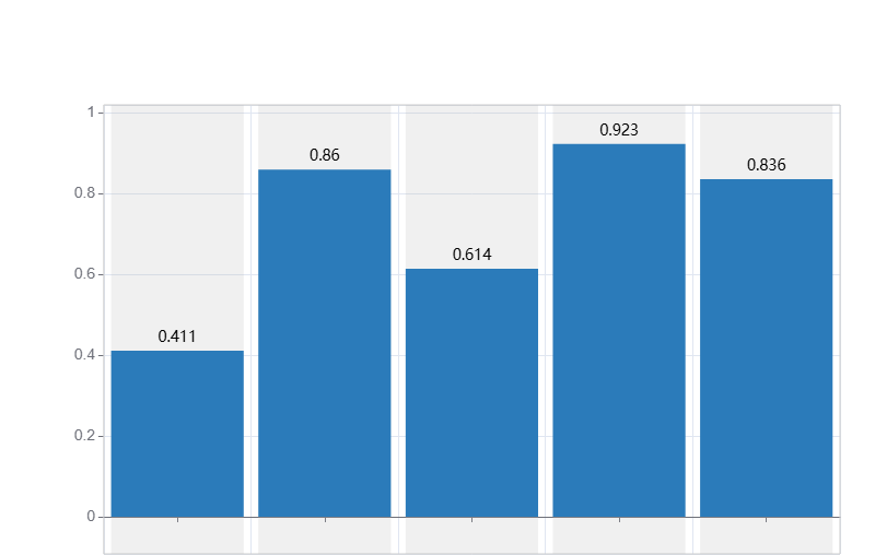

The headline 0.81 splits apart. Most clusters are fine. But three of them — the kernel ranks them clearly — are where the model is thin, and one is genuinely broken: in that pocket the monotone model’s ranking is barely better than a coin, in places worse. The average was true and misleading at the same time, exactly as before.

Where does the weak pocket sit? Take the weakest cluster against the rest and rank the features by PSI, the same population-stability index risk teams use for drift — pointed inward this time, one cluster versus its complement:

drift = ds.data_drift_test(dataset1="train", sample_idx1=np.where(in_weak)[0],
                           dataset2="train", sample_idx2=np.where(~in_weak)[0],
                           distance_metric="PSI")
drift.plot("summary")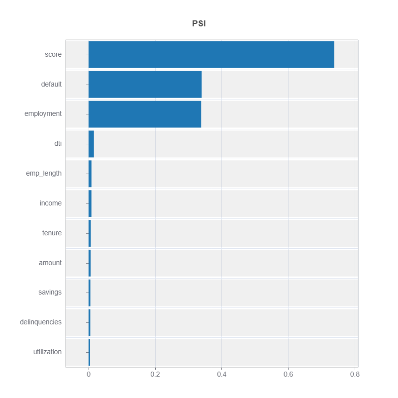

One feature towers over the rest: credit score (PSI ≈ 0.74, far past the 0.25 “large shift” line; nothing else clears 0.02). Overlay the score distribution of the weak cluster against the rest and the shift stops being a statistic and becomes a picture:

top = drift.table.index[0]           # highest-PSI feature -> "score"
drift.plot(("density", top))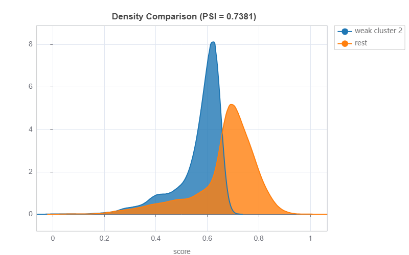

The weak region is a low-score pocket — applicants bunched a full band below everyone else, where the monotone model’s leaf geometry does not carve finely enough. We did not go looking for it with a hunch. The model’s own kernel surfaced it, and PSI named it.

Now we act on the map. Instead of one global model straining to be good everywhere, a Mixture of Experts (https://modeva.ai/docs/2-user-guide/models/moe) trains several specialists and lets a gate route each applicant to the ones that serve its region best. The prediction is a gate-weighted blend of the experts,

where beta_g(x) is the (calibrated) probability that applicant x belongs to region g. An expert whose region lands on the weak score pocket gets to specialize there, while the experts covering the healthy regions keep doing what already worked.

The one rule the repair may not break is the one that got us here: every expert must stay monotone. In Modeva that is a single constructor away — the same constraint string flows into each expert:

moe = MoMoEClassifier(n_clusters=5, expert="catboost",
                      depth=2, monotone_constraints=mono)
moe.fit(ds.train_x, ds.train_y.ravel())

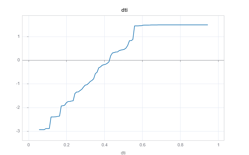
Because every expert is a monotone depth-2 CatBoost, the mixture is still a monotone, functional-ANOVA model. The gate-averaged effects come out with the same clean shapes — dti still strictly increasing, score still strictly decreasing — so nothing we built in the first three sections is thrown away.

A higher headline number is only convincing if the lift shows up in the weak regions and leaves the healthy ones alone. So re-use the kernel’s cluster labels and compare per-cluster test AUC, base model versus mixture of experts:

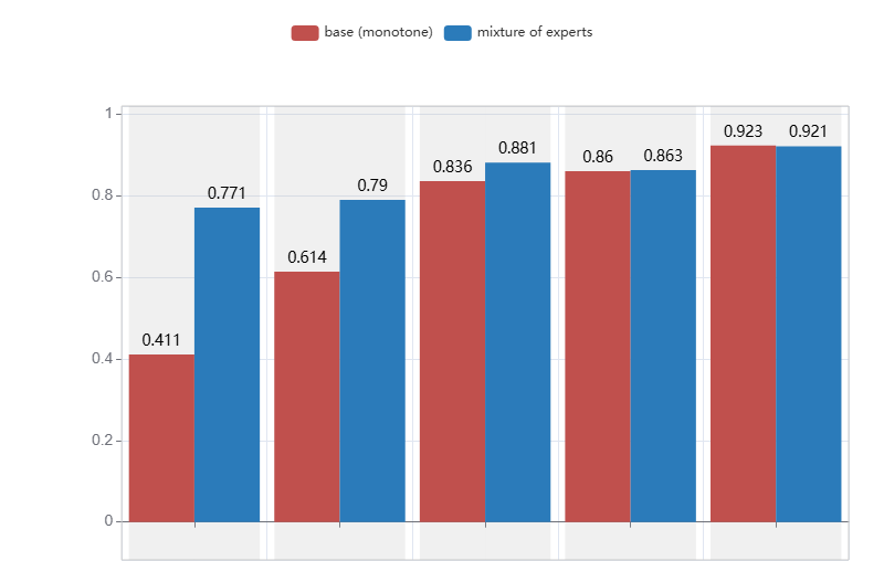
The repair is surgical. The two clusters the kernel flagged as weakest — where the base model scored 0.41 and 0.61 — jump to 0.77 and 0.79. The cluster that was essentially inverted is now a working classifier. The strong clusters, at 0.86 and 0.92, do not move. The effort went exactly where the model was failing and nowhere else.

And the tax we came to recover? The single monotone model was 0.81; the free black box, 0.92. The monotone mixture of experts lands at about 0.88 — closing roughly two-thirds of the gap to the unconstrained model without ever leaving the monotone, interpretable family. That is the whole trade of this chapter: you do not choose between a model you can defend and a model that performs. You build the defensible one, let its kernel tell you where it hurts, and send experts to exactly those places.

Everything above is a handful of first-class calls in Modeva — the local CSV load, the cross-validated monotone CatBoost, the FANOVA read-out, the leaf kernel, the Nyström weakness map, the PSI, and the monotone mixture of experts. It is free: generate a licence and install in one line at modeva.ai.

# pip install modeva  (free licence key at https://modeva.ai/)
from modeva import DataSet, TestSuite
from modeva.models import (MoCatBoostClassifier, MoFuseKernelClassifier,
                           ModelTuneGridSearch, MoMoEClassifier)
ds = DataSet(); ds.load_csv("credit_default.csv")
ds.set_target("default"); ds.set_task_type("Classification")
ds.set_random_split(test_ratio=0.2, random_state=0)
ds.scale_numerical(features=tuple(ds.feature_names), method="minmax"); ds.preprocess()
# monotone_constraints as a POSITIONAL STRING in feature order:
# +1 increasing, -1 decreasing, 0 free — one per driver.
mono = "(" + ",".join(str(direction[f]) for f in ds.feature_names) + ")"

The companion notebook runs top to bottom on the full dataset: tune the depth-2 CatBoost, contrast the free and monotone effect shapes, read the model with FANOVA, build the leaf kernel, draw the per-cluster weakness map, name the weak region with PSI, and repair it with a monotone mixture of experts — checking the lift lands where the kernel said it would.

▶ Run it in Colab (no install): open in Colab

📦 Notebook and data: github.com/asudjianto-xml/MRM/tree/main/Tabular/02-mixture-of-expert/notebooks

🔑 Get Modeva (free): https://modeva.ai/

The previous installment, Trees Are Kernels — and the Kernel Knows Where the Model Is Weak, is where the weakness map comes from; start there if you want the diagnosis before the cure. This chapter is what you do once you have the map.

Post 4 gave us the map: a boosted model’s own kernel, showing where it fails. Post 5 spent it. A model you can defend costs accuracy — but not as much as it first appears. Build the monotone, interpretable model; read it with functional ANOVA; let its own kernel mark where it is weak; then send monotone experts to precisely those regions. You buy back most of the performance and break none of the guarantees. Trees knew where the model was weak — and now you know how to repair it in place.

The Learned Kernel is a free weekly series. The posts carry the intuition and the runnable code; every example runs on Modeva — modeva.ai.