The Model That Scores Its Own Geometry

Chapter 5 of The Learned Kernel. Last time we saw that a gradient-boosted ensemble is secretly a kernel machine (https://agussudjianto.substack.com/p/trees-are-kernels-and-the-kernel), with a similarity it learned from the labels. But boosting learns that similarity greedily, split by split, and never writes down a number for how good the resulting geometry is. This chapter produces that number. It turns out to be the hinge the rest of the book swings on.

Take one block in the California housing data and ask three models for its median house value. A linear model gives a point. A boosted ensemble gives a point. A Gaussian process gives a point and a range: say $230k, give or take $40k, with the range wider for a block out in a sparse rural corner than for one in a dense suburb. That range is not a bolt-on. It comes out of the same computation as the prediction, at no extra cost. And it is the least of the three things a Gaussian process gives you from one idea.

The idea is a single identification. A kernel is a covariance, and a covariance is a prior over functions. Accept that and three things follow. The prediction you get back is exactly the kernel ridge regression from two chapters ago. The uncertainty comes attached for nothing. And the kernel picks up a score, one number that says how well this geometry explains the data. The third one is what matters. A geometry with a score is a geometry you can learn by climbing the score, and climbing the score is what “learn the kernel, don’t choose it” actually means once you have to do it.

The move is this. Instead of fitting one function to the data, put a probability distribution over functions and let the data sharpen it. A Gaussian process is the natural distribution to use. Pick any handful of input points and the function’s values at those points are jointly Gaussian, with covariance given by the kernel. In symbols:

So the kernel is no longer a similarity we asserted by hand. It is the prior covariance of an unknown function. If the kernel says two blocks are similar, the prior says their house values move together. Everything geometric about the kernel, how far its influence reaches and how wiggly a function it will tolerate, shows up in the shape of the functions the prior prefers.

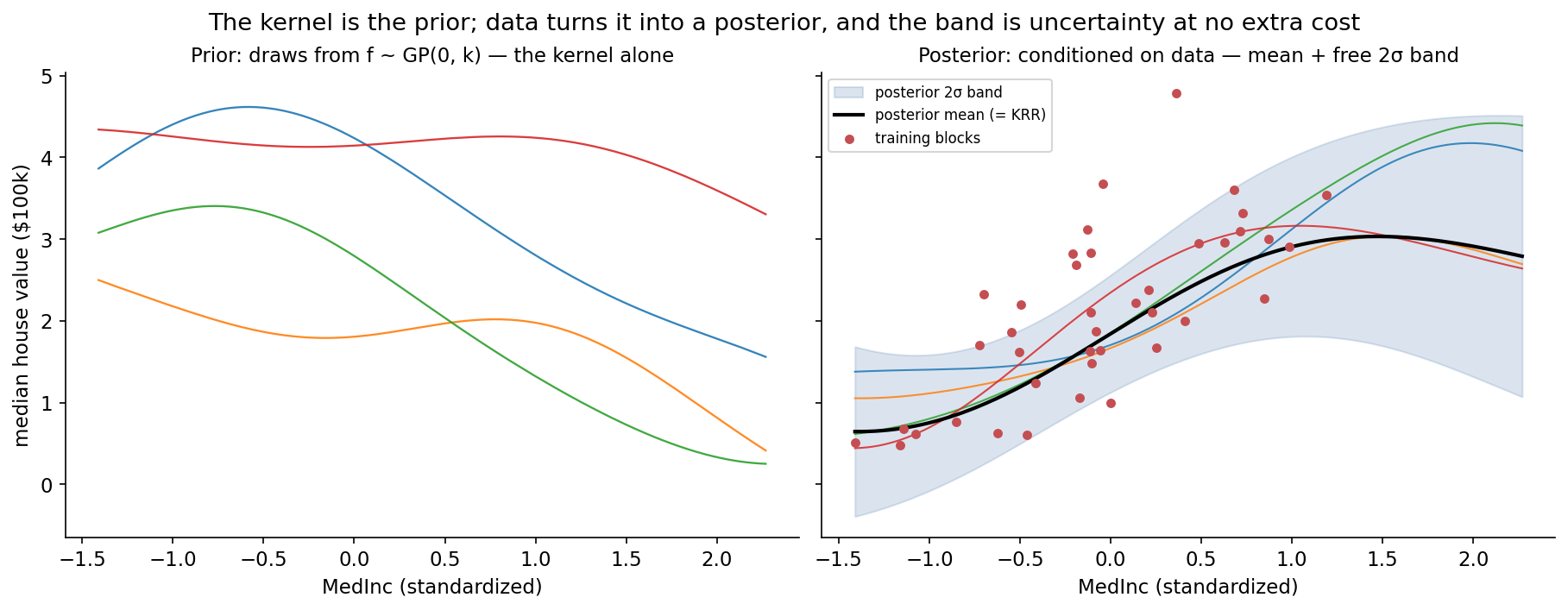
The left panel shows four functions drawn from the prior along a slice of the median-income axis. They are smooth and wandering, held back by nothing. That is the kernel talking before it has seen any data. The right panel conditions on a handful of training blocks. The functions snap to the data, the spread collapses near the observations, and the shaded band, which is the posterior’s two-sigma uncertainty, pinches tight where blocks cluster and flares wide past the edge of the data. The kernel was the prior. The data turned it into a posterior. The band is the uncertainty, and we did nothing extra to get it.

What the kernel controls in that left panel is everything that follows. Make the length scale short and the prior draws turn jagged, changing direction within a fraction of an income unit. Make it long and they go lazy, barely bending across the whole axis. The amplitude sets how far they swing up and down. Choosing a kernel is therefore choosing a belief about the unknown function before you have seen a single label: how smooth it is, how large its swings are, which directions in feature space carry the signal. A classical kernel method makes you pick that belief by hand and live with it. This chapter is about not having to. The data can tell you which belief it prefers, through a number we are about to meet. Before that number, though, one question we have been skating over: why is a kernel allowed to be a covariance in the first place?

A Gaussian process is defined entirely through its finite pieces. Name any finite set of input points and the values of f at those points follow a multivariate Gaussian. A multivariate Gaussian is pinned down by two things, a mean vector and a covariance matrix. Set the mean to zero and the covariance matrix is all that is left to choose. So building a GP comes down to one question: given points x₁ through xₙ, what covariance matrix do we place on f(x₁) through f(xₙ)?

The kernel answers it. Fill entry (i, j) of the matrix with k(xᵢ, xⱼ). For that to be a covariance matrix at all it has to pass two tests, and both are the conditions we already demanded of a kernel in Chapter 2. Covariance is symmetric, since Cov(a, b) = Cov(b, a), so we need k(x, x’) = k(x’, x). And no combination of the outputs may have negative variance: for any weights c, the variance of Σᵢ cᵢ f(xᵢ) works out to cᵀKc, and a variance cannot fall below zero, so we need cᵀKc ≥ 0. Symmetric and positive semidefinite. That pair is the definition of a positive-semidefinite kernel.

So the identification is not sleight of hand. The valid covariance functions and the PSD kernels are one and the same class, reached from two directions. Probability arrives at it by refusing negative variances. Inner-product geometry arrives at it through Mercer’s theorem, which writes the same symmetric PSD function as k(x, x’) = ⟨φ(x), φ(x’)⟩ for some feature map φ. A kernel is at once an inner product in a feature space and a covariance over function values, because those are the same condition in different clothes. Chapter 2 built the object as geometry. The Gaussian process reads the very same object as probability.

And the reading is the natural one. Covariance measures how strongly two quantities move together, and the kernel measures how similar two inputs are, so setting them equal is just the statement that similar inputs have outputs that move together. When k(x, x’) sits near its maximum the two house values are almost perfectly correlated, and learning one nearly fixes the other. When k(x, x’) is near zero the two are close to independent and one tells you little about the other. That is the smoothness assumption every model leans on in order to generalize, written in the language of correlation rather than distance.

That leaves one honest worry. We specified the distribution only on finite sets of points, yet we want a distribution over whole functions. Does that add up? It does, as long as the finite Gaussians agree wherever they overlap, meaning that if you drop a point the smaller Gaussian left behind is the one you would have written down directly. Gaussians are closed under that kind of marginalization and the kernel’s Gram matrices are consistent by construction, so the agreement holds on its own. The positive-semidefinite condition keeps each finite Gaussian well-defined, and that consistency stitches them into a single prior over functions.

Conditioning a joint Gaussian on part of itself has a closed form. No optimization, no iteration. Run it and the posterior mean at a new point x comes out as

where K is the kernel matrix on the training points, K_* is the row of kernel values between x and the training points, and σ² is the noise variance. Set α = (K + σ²I)⁻¹y and this reads m(x) = Σᵢ αᵢ·k(x, xᵢ), a weighted sum of kernel evaluations against the training set.

If you read Chapter 2, that is kernel ridge regression, the same predictor down to the letter. The only new thing is the name of the regularizer. Where ridge regression had a knob λ you tuned by cross-validation, the Gaussian process says:

> the ridge λ is the observation-noise variance σ².

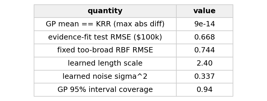
The probabilistic object and the regularized-least-squares object are the same machine. On California I computed the GP posterior mean by hand from the Gaussian conditioning identity, computed kernel ridge regression with scikit-learn and subtracted the two. The largest disagreement anywhere in the test set is about 9 × 10⁻¹⁴, which is machine zero.

What the GP adds on top is the variance, v(x) = k(x,x) − K_(K+σ²I)⁻¹K_ᵀ. Look at the shape of it: the prior variance, minus a reduction that is large only where x correlates strongly with the training data. Far from any training point K_* → 0 and the variance climbs back to the prior. The model widens its interval precisely where it has no evidence. Kernel ridge regression and trees hand you a point and stop. The GP hands you a point and a measure of how far to trust it.

That measure is not a formality. On California the posterior variance runs from about 0.002 for a block inside a dense cluster of training data up to the full prior value of 1.0 for a block off in an unobserved corner of feature space. That is a factor of five hundred between “we have seen many blocks like this one” and “we are guessing.” Anything downstream that has to price risk, whether a lending decision or a safety check, needs exactly that distinction, and here it falls out of the same matrix factorization that produced the prediction. No bootstrap, no ensemble, no held-out resampling. One Cholesky decomposition gives you both the answer and the confidence in it.

This is the part the whole book turns on. We have a kernel, but its parameters, the length scale and the noise, are still unset. We want a number that tells us how good a given choice of them is. The Gaussian setup hands one over. Integrate the unknown function out of the model and what is left is a plain Gaussian for the data itself, y ~ N(0, K + σ²I). The probability this puts on the data you actually observed is the evidence. Its logarithm is

Two terms are worth reading. The first, −½ yᵀA⁻¹y, is a fit term. It is large when the covariance A accounts for how the data spreads out. The second, −½ log|A|, is a complexity penalty. |A| measures how much volume the covariance occupies, so a flexible, sprawling kernel is charged here. Fit pulls one way and complexity pulls the other. Their balance is Occam’s razor written as a formula, and it is differentiable, which is the part that will matter.

This is the number boosting never had. A boosted ensemble learns its geometry greedily, and the only verdict on it is the training loss. The Gaussian process scores the geometry directly, with a quantity you can compute and differentiate. A score you can differentiate is a score you can climb.

The complexity term rewards a second look, because it does by arithmetic what cross-validation does by brute force. log|A| is the log-volume of the ellipsoid the covariance traces out. A kernel with a long length scale is rigid. It can only express slowly-varying functions, so its ellipsoid is thin and log|A| is small. A kernel with a short length scale can express almost anything, so its ellipsoid is fat and log|A| is large. The evidence charges a kernel for its own flexibility this way, on its own, without ever holding out a validation set. A rigid kernel that happens to fit is rewarded twice, once for the fit and once for being simple, while a flexible kernel has to fit well enough to earn back the volume it pays for. Occam’s razor, done in arithmetic.

So we maximize the evidence over the kernel’s parameters, the length scales, the amplitude and the noise, by gradient ascent. It has a name, ML-II or empirical Bayes, but the picture is plain. Turn the dials on the geometry until the data is as probable as it can be. Do it with one length scale per feature and you have recovered automatic relevance determination from Chapter 3. The relevances are the length scales the evidence settles on.

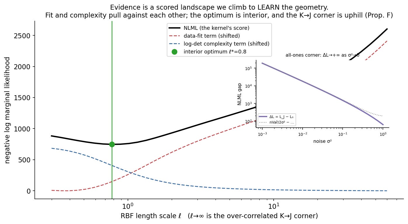
The main panel scans the evidence over the RBF length scale on California. The fit term rises to the right, the complexity term falls to the right, and the negative log marginal likelihood, the thing we minimize, bottoms out at an interior optimum around ℓ ≈ 0.8. Not at zero and not at infinity, but in the middle, where fit and simplicity settle their bargain. Let scikit-learn run its optimizer over both the length scale and the noise and the evidence-fit kernel reaches a test RMSE of 0.668 on California. That beats a deliberately too-broad hand-set kernel at 0.744, and its 95% intervals cover 94% of held-out blocks. The geometry was fit, not tuned. There was no grid to search.

There is an objection that has to be answered, and it is a real one. Ober, Rasmussen and van der Wilk raised it in 2021. Look again at the complexity penalty, −½ log|A|. A devious optimizer could shrink |A| without finding any real structure, just by making every point look similar to every other, driving the kernel toward the all-ones matrix with every off-diagonal equal to 1. That matrix has the smallest volume there is. If the evidence rewarded it, then “the score makes the kernel learnable” would be hollow, since the score could be gamed into a useless over-correlated blob.

It cannot, and the reason is a clean cancellation. Call the all-ones kernel J. Because J has a single nonzero eigenvalue, its pieces have closed forms. For instance log|J + σ²I| = log(n+σ²) + (n−1)·log σ². Plug those into the evidence and compare J against any kernel that genuinely fits. As the noise σ² shrinks, which is the regime the collapse itself drives you into, the gap in the negative log marginal likelihood is

The over-correlated kernel does save on the complexity term, but only by log(1/σ²). It pays for its ruined fit by 1/σ², because a kernel that calls everything similar can only predict the global average, and the noise model is charged for every bit of variance it misses. 1/σ² beats log(1/σ²) every time. So the gap does not shrink toward zero. It blows up. The all-ones kernel is not a low point of the evidence. It is a hill the optimizer rolls off.

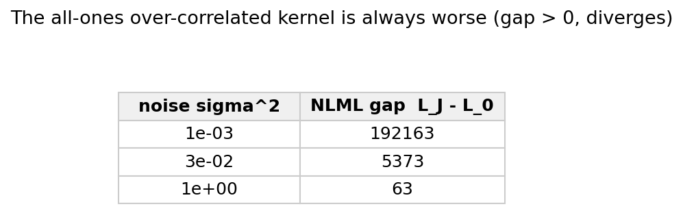
I checked this on California numerically. The closed forms match the exact eigenvalue computation to eleven and thirteen decimal places, and the evidence gap to the all-ones kernel is positive at every noise level, growing from about 63 at σ²=1 to roughly 190,000 at σ²=0.001. Taiwan Credit gives the same picture. For this bounded geometry, the collapse the critique worried about is uphill.

You can see the same thing without any algebra in the landscape of the main figure. The over-correlated corner is the far right, where the length scale ℓ → ∞ and every block looks like every other. The negative log marginal likelihood does not dip toward that corner. It climbs steadily away from it. An optimizer dropped anywhere on the curve rolls toward the interior optimum and away from the all-ones corner, because the corner is a ridge and not a valley. The move that would shrink the complexity penalty is the same move that wrecks the fit, and the fit term wins that trade by a widening margin as the noise drops. So when scikit-learn’s optimizer runs free over the length scale and the noise, it settles at a sensible interior geometry every time rather than a degenerate blob. That is what makes “learn the kernel by climbing its score” a safe instruction instead of a trap.

There is a deeper reason it is harmless, and the book proves it in full. The only parameters that drive the kernel toward all-ones are the same ones that flatten the predictor to the global average. Collapsing the geometry and destroying the fit are one move, not two. You cannot get one without the other, so the optimizer never wants either.

Three chapters ago we said the geometry should be learned and not chosen, and we have been circling what “learned” really means ever since. Boosting learned a kernel greedily. The Gaussian process gives the cleaner answer. A kernel is a covariance, a covariance scores itself through the marginal likelihood, and learning the kernel is climbing that score. The prediction you get for free is the kernel ridge regressor. The uncertainty you get for free is the posterior band. And the result that makes the climb trustworthy is that the score cannot be gamed into a degenerate blob. Every later chapter runs on this engine, the spectral kernels and the amortized in-context learners alike: score the geometry, then climb the score.

The whole identity is a few lines. Compute the GP mean by hand, compute kernel ridge with scikit-learn and check that they agree:

A   = rbf_kernel(Xtr, Xtr, gamma=gamma) + sigma2 * np.eye(n)   # K + sigma^2 I
cho = cho_factor(A, lower=True)
alpha   = cho_solve(cho, y_centered)                           # (K + s2 I)^-1 y
gp_mean = rbf_kernel(Xte, Xtr, gamma=gamma) @ alpha + ybar     # m(x) = K_* alpha
krr = KernelRidge(alpha=sigma2, kernel="rbf", gamma=gamma).fit(Xtr, y_centered)
assert abs(gp_mean - (krr.predict(Xte) + ybar)).max() < 1e-6   # ~ 9e-14

The companion notebook draws the prior and posterior, asserts the GP-mean = KRR identity to machine precision, scans the evidence landscape and lets you move the noise to watch the optimum stay interior instead of running off to the over-correlated corner.

▶ Run it in Colab (no install): open in Colab

📦 Code: github.com/asudjianto-xml/Learned-Kernel

The previous installment, Trees Are Kernels — and the Kernel Knows Where the Model Is Weak, is where the greedy score-free way of learning a kernel comes from, the contrast this chapter answers.

A kernel is a covariance. A covariance scores itself through the marginal likelihood. Learning the kernel is climbing that score. The prediction is kernel ridge regression, the uncertainty is free, and the climb is safe, because the geometry cannot collapse into a blob to cheat the score. That is the engine the rest of the book runs on. Next time: what every prediction is actually made of, and the case-based evidence sitting behind the number.

The Learned Kernel is a free weekly series adapted from my upcoming book of the same name. The posts carry the intuition and the runnable code; the book carries the full derivations.