The Geometry Hidden in Every Model

This is the first post in The Learned Kernel, a weekly series that builds one idea, chapter by chapter: learning is the discovery of geometry, the kernel is what carries it, and the kernel should be learned, not chosen. Every post runs on real data, and the full, executed code is one click away at the end.

Pick one California census block and ask three different models what its houses are worth. A ridge regression says $306k. A regression tree says $370k. A thirty-nearest-neighbor rule says $321k. Same block, same data, three numbers.

The usual way to read this is that we have three competing methods and a model-selection problem to solve. That reading misses what is actually going on. Each of those three numbers is built the same way. Each is an average of house values the model has already seen, with one model’s average leaning on one set of past blocks and another’s leaning on a different set. The methods do not disagree about arithmetic. They disagree about which past blocks count when you stand at this one.

That disagreement is the subject of this series. By the end of this post I want one idea to feel obvious: every supervised model, whatever its surface form, answers a query by combining the labels it was trained on, and the weights it places on those labels are a geometry — a precise statement of which points the model treats as near and how influence falls off with distance. Learning is the discovery of that geometry. And the object that writes the geometry down has a name we will earn carefully over the coming weeks: the kernel.

Why start here, with something so elementary? Because the habit this series is built to break is invisible until you name it. We are trained to think of a model as a box that maps inputs to outputs, and of “which model” as a menu choice — tree, or linear, or neural net. But the choice that actually decides the answer is the one underneath: the model’s notion of similarity, the shape of “near.” Once you see that every model carries such a notion, two questions become unavoidable. Where did that geometry come from? And could we do better by learning it from the data instead of inheriting it from the algorithm? Those two questions are the whole book. This first post just makes the geometry visible, so we have something concrete to learn.

Hold out one block from the California Housing data and predict its median house value. The block sits in the Los Angeles basin: median income around $59k, houses about 37 years old, a bit under six rooms each. Train three familiar models on the other twenty thousand blocks and ask each for a number.

Look at what each model actually computes. The ridge regression forms a coefficient vector and takes a dot product with the query’s features. The tree drops the query down its branches to a leaf and reports the average value of the training blocks in that leaf. The neighbor rule finds the thirty most similar blocks and averages their values. Three different procedures — but every one of them returns a combination of training labels. The tree literally averages labels. The neighbor rule literally averages labels. And the ridge prediction, once you substitute its fitted coefficients back in, is also a weighted sum of training labels, just with weights that are less obvious to the eye.

This is not a coincidence of these three models. It is the shape of supervised prediction itself. Write the common form once:

The prediction at a query x is a weighted vote over the n training labels yᵢ, and the function wᵢ(x) — how much training case i counts toward the answer at x — is the influence of case i on the query. Every model fits this template. They differ in one thing only: which cases get weight, and how much. So if we want to compare models, we should stop comparing their predictions and start comparing their weights.

Here are the three predictions for our Los Angeles block, with the identity checked on the data and the number of training blocks each model actually used:

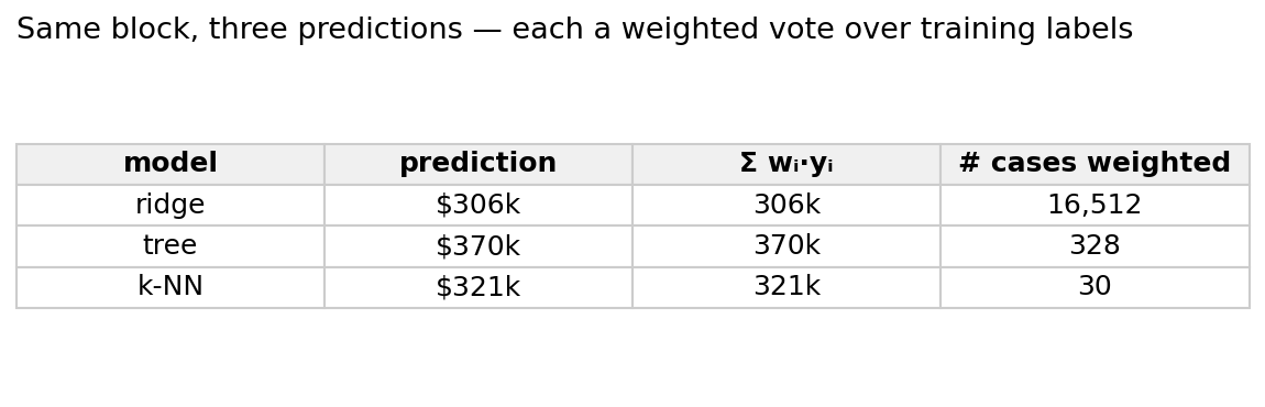
Read the last column. Ridge places weight on all 16,512 training blocks. The tree uses only the few hundred in its leaf. The neighbor rule uses exactly 30. Three numbers within $64k of each other, built from completely different sets of cases. The middle column is the punchline of this section: Σᵢ wᵢ·yᵢ reproduces each model’s own prediction exactly. The weighted-vote identity is not a metaphor. It holds on the data, to machine precision.

The weights are not abstract. We can compute wᵢ(x) for each model and look at it, and each one turns out to have a recognizable shape.

Ridge. Substitute the fitted coefficients back into the prediction and the weight on case i comes out as

This is a bilinear form in x and xᵢ. Two things follow. The level sets of equal influence are ellipsoids, stretched along the directions the data deem important and squeezed along the rest — influence has preferred directions, it is not the same in every direction. And the weights are signed and global: every training block gets some weight on this single query, and many of those weights are negative. Ridge reaches across the entire state to answer a question about Los Angeles.

Regression tree. The tree sends the query to a leaf and averages the labels there:

Every weight inside the leaf is equal and positive, every weight outside is exactly zero. The influence is a flat box: uniform inside, sharply zero at the edge, and — because a tree splits one feature at a time — axis-aligned. The tree consults a few hundred blocks it judged similar and ignores the other sixteen thousand completely.

k-nearest-neighbors. The neighbor rule keeps the k closest blocks and averages them:

With k = 30 each neighbor gets weight 1/30, and everything else is silent. The influence is an isotropic ball: round, uniform inside, zero outside, centered on the query.

Three weight functions, three pictures of “near.” The figure below shows the influence each geometry would assign to a hypothetical block at every location on the map: ridge a smooth, signed gradient that spans the state; the tree a hard axis-aligned box; the neighbor rule a round patch.

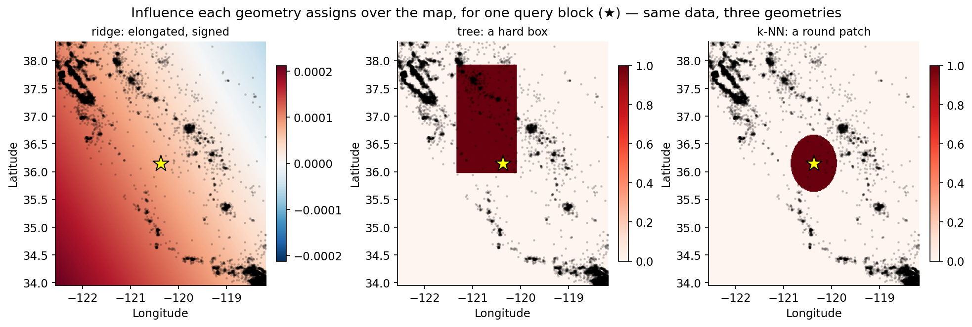
These pictures are not decoration. They are the models’ geometries — the precise sense in which each model decides what counts as similar. And they explain the three numbers we started with. A signed statewide reach, an axis-aligned box and a round local patch are three different answers to “which blocks are like this one.”

Each shape is good at one thing and bad at another, and the rest of the series lives in those trade-offs. The ellipse adapts to correlations between features — it can learn that income and house age matter in a particular combined direction — but it is one global shape, the same everywhere, so it cannot bend to local structure. The box is the opposite: it adapts locally and snaps to sharp thresholds, which is exactly why gradient-boosted trees win on tabular data with hard cutoffs, but its predictions are flat inside each cell and jump at the edges, so it cannot represent a smooth trend without staircasing. The ball is the simplest and most honest about locality, but it is isotropic — it treats every direction as equally important, which is rarely true. None of the three is wrong. Each is a different bet about where the structure in the data lives. The trouble is that all three bets were placed before anyone looked at this particular target.

We can also ask each model which specific blocks it leaned on hardest. The cases with the largest weight tell the same story from the other side:

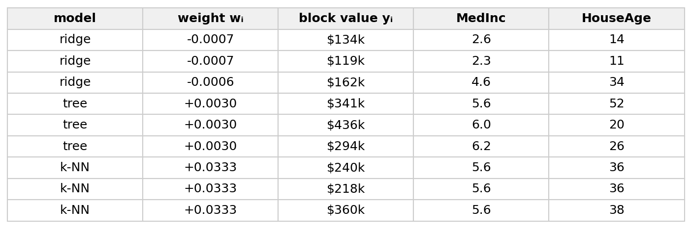
Ridge’s heaviest cases are signed and extreme — low-income blocks pulling the estimate down with negative weight, the value-capped richest blocks pulling it up — drawn from across the state. The tree’s and the neighbor rule’s are all positive and local: nearby blocks that simply look like the query. Same target, three completely different notions of evidence.

The same structure shows up on a classification problem, with one small twist. Take one applicant from a credit-default dataset and ask whether they will default. The tree routes the applicant to a leaf and reports the fraction of that leaf that defaulted; the neighbor rule reports the fraction among the most similar applicants. Both are still Σᵢ wᵢ(x)·yᵢ, now voting over a 0/1 label. The weighted-vote identity holds across regression and classification because it is a fact about the form of these predictors, not about the target.

Step back from the three formulas. In every case the weight wᵢ(x) measures one thing — how much the training point xᵢ counts when we predict at x — and that quantity deserves a name. Call it k(x, xᵢ): a function of two points that says how much the second should count toward an answer at the first. No deep machinery yet. Just the plain idea that this function is the model’s notion of similarity, written once.

Once we name it, the three models line up under a single template. Normalize the similarity so the weights sum to one and you get

The tree is this template with a hard kernel k(x, xᵢ) = 1 if xᵢ falls in the same leaf as x, and 0 otherwise. The neighbor rule is the same template with k(x, xᵢ) = 1 if xᵢ is among the k nearest, and 0 otherwise. Both are blunt, 0-or-1 similarities — you are either in the box or out of it, a neighbor or not. Ridge does not normalize and its weights can go negative, but its bilinear form is a kernel too, the linear kernel k(x, xᵢ) = xᵀM xᵢ with M = (XᵀX + λI)⁻¹, once we agree to read the features through a linear map. The only reason ridge does not look like a smoother on the raw inputs is that its similarity lives in a transformed feature space — which is exactly the move the next post makes precise.

So the kernel is the common denominator. Choosing a model is, underneath, choosing a kernel. Which raises the question this whole series is about: where should the kernel come from?

The classical answer is to choose it. Open a course on kernel methods and the first thing you do is pick one — Gaussian, polynomial, Laplacian — fix its bandwidth and proceed. Everything downstream lives inside that choice, and the geometry is frozen before the data are consulted. The kernel is an assumption.

This series takes the opposite stance, and the reason is already on the page. The kernel is the model’s geometry, and the geometry is the very thing we are trying to learn — which blocks are like this one, in which directions, at what scale. A thing you are trying to learn cannot also be an input you fix in advance. It has to be discovered from the data, shaped by the same process that produced the data. That is the inversion everything turns on: the kernel is not chosen, it is learned.

One of our three models already broke the classical habit, and that is the clue. The tree’s box was not handed to it. The splitting rule fit those boundaries to the labels, placing cuts where they reduced error, so the tree’s geometry was learned from data — the first learned kernel we will meet. Ridge and the neighbor rule did not go nearly as far. Ridge fixes its similarity to a single global linear form; the neighbor rule fixes a round ball and only tunes its radius through k.

You can feel how arbitrary that fixed knob is by turning it. For our block the neighbor rule predicts $238k at k = 1 — a single noisy comp — then $284k at k = 5, $321k at k = 30, $308k at k = 200, $289k at k = 1000, and on down toward the global mean of $207k as k swallows the whole state. The number you report is a direct function of a radius you picked by hand. Nothing in the data told us which k is right. We chose it. The rest of the series is about replacing that choice with a geometry the data actually earn — a radius, a shape, a set of directions, all fit by a criterion rather than a default.

There is also a warning hidden in the three pictures, and it is the one that makes “just learn the kernel” harder than it sounds. The same prediction can come from very different weights. Ridge and the neighbor rule landed within $15k of each other on our block, yet their weight vectors barely resemble each other — across the training set the two sets of weights correlate at just 0.07, and a quarter of ridge’s are negative where every one of k-NN’s is positive. Two models, nearly the same answer, almost orthogonal geometries. Predictions agreeing does not mean geometries agreeing. So the fit alone does not pin the geometry down, which means learning the kernel will require a criterion that scores the geometry itself, not just the predictions it produces. That criterion is where this series is headed.

Everything above is a few lines of code. Here are the three weight functions, exactly as used to make the figures — each one returns the vector of weights wᵢ(x) a model places on the training set for a query x:

⬛ SUBSTACK CODE BLOCK (python) — paste the code below:

def ridge_weights(Xtr, x, lam):     # wᵢ = xᵀ (XᵀX + λI)⁻¹ xᵢ  — global, signed
    Xb = np.hstack([Xtr, np.ones((len(Xtr), 1))]); xb = np.append(x, 1.0)
    return xb @ np.linalg.solve(Xb.T @ Xb + lam * np.eye(Xb.shape[1]), Xb.T)
def tree_weights(tree, Xtr, x):     # wᵢ = 1{same leaf} / leaf_size  — a hard box
    same = (tree.apply(Xtr) == tree.apply(x[None])[0]).astype(float)
    return same / same.sum()
def knn_weights(knn, Xtr, x, k):    # wᵢ = 1/k on the k nearest  — a round patch
    idx = knn.kneighbors(x[None], k, return_distance=False)[0]
    w = np.zeros(len(Xtr)); w[idx] = 1.0 / k; return w

The companion notebook fits the three models on California, computes these weights, and asserts on the data that each model’s own prediction equals Σᵢ wᵢ(x)·yᵢ to machine precision. It also gives you a slider to move the query block and turn the three knobs — k, tree depth, ridge λ — and watch the box, the disk and the gradient change shape in real time.

▶ Run the notebook in Colab (no install): https://colab.research.google.com/github/asudjianto-xml/Learned-Kernel/blob/main/notebooks/ch01_geometry_hidden.ipynb

📦 Code: https://github.com/asudjianto-xml/Learned-Kernel — pip install learned-kernel

Notebook: https://github.com/asudjianto-xml/Learned-Kernel/blob/main/notebooks/ch01_geometry_hidden.ipynb

If you have read my earlier post, [What Is the Prediction Actually Made Of? https://agussudjianto.substack.com/p/what-is-the-prediction-actually-made], this is the idea it rested on, now made the starting point of a longer argument.

Every model induces a geometry. The good ones learn it. And once the geometry is the explicit object of the method, the model becomes something you can read — its relevances, its interactions, the very cases it leaned on. That is where this series is going, and it is what will make a learned kernel not only accurate but trustworthy. Next week: why smoothing, ridge regression, the support vector machine, the Gaussian process and even attention are all one machine reading one kernel.

The Learned Kernel is a free weekly series adapted from my book of the same name. The posts carry the intuition and the runnable code; the book carries the full derivations. Subscribe to follow the whole argument from gradient-boosted trees to in-context learning.