Geometric Algebra for Causal Discovery: Sector Rotation May Be a Market Bet in Disguise

This is part of a series on geometric algebra, used not as an abstract formalism but as a way to read real multivariate systems. Here it meets a familiar investing question. Is sector rotation a real cross-sector signal, or a market effect that only looks like one?

Sector rotation has an intuitive story. Growth-sensitive sectors respond first to changing conditions: technology, consumer discretionary and industrials. Defensive sectors follow: staples, health care and utilities. If that sequence reliably lasts a day or two, you could trade it. Use today’s move in growth to position for tomorrow’s move in defensives.

The problem is that a lead-lag is not yet a causal mechanism.

Two groups can move in sequence because one drives the other. They can also move in sequence because both respond to the same market-wide force at different speeds. In a lagged-correlation chart these look the same. For a portfolio they are not. The first is an independent cross-sector signal. The second is exposure to the market factor, arriving on a lag.

Our study, Is Sector Rotation Causal? A Geometric Test of the Growth-to-Defensive Lead-Lag, tests that distinction on eleven U.S. sector ETFs from November 2020 through October 2025. The finding is clean:

The growth-to-defensive rotation is there before adjustment and gone after conditioning on the common market factor. It is a market-driven, stress-regime pattern, not a standing cross-sector effect.

The point is not really about one trading rule. It is a discipline for factor research. Before you treat a lead-lag as alpha, check what is left once the shared driver is removed.

We compare three growth sectors against three defensive sectors. Growth is Technology (XLK), Consumer Discretionary (XLY) and Industrials (XLI). Defensive is Consumer Staples (XLP), Health Care (XLV) and Utilities (XLU). That gives nine growth-defensive pairs. For each pair we ask one question. Do today’s growth returns help predict tomorrow’s defensive returns more than the reverse does?

With no adjustment, all nine pairs point the conventional way: growth leads defensive, with an average gap of +0.133. Then we add controls in stages. The effect’s own prior-day return leaves it intact. A time-shuffled market factor, which keeps the market’s distribution but scrambles its timing, also leaves it intact. Then we add the real, time-aligned market factor, and the gap falls to +0.008, with only four of the nine pairs still leaning growth-first.

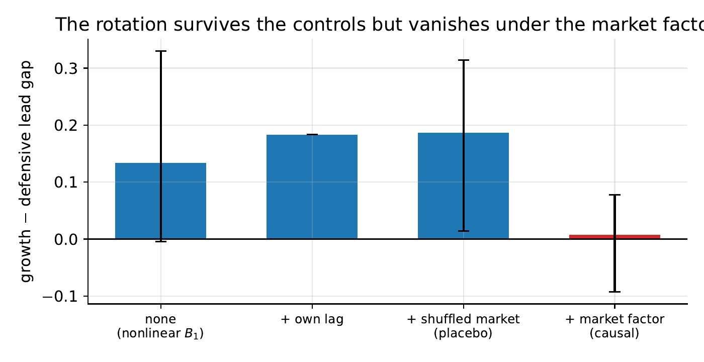
The growth-minus-defensive lead gap under each control, with 90% block-bootstrap intervals. It holds under the own-lag and shuffled-market controls, then drops to zero under the aligned market factor.

The last step is the one that matters. The control is an equal-weight average of the other nine sector returns. It is built separately for each pair, so neither tested sector sits inside its own control. The placebo step matters just as much. A time-shuffled market series keeps the same distribution but loses the timing, and it leaves the rotation intact. So the real market factor does not kill the pattern because it is one more flexible control. It kills it because its timing is what the apparent signal was tracking.

Correlation and lagged correlation are useful descriptions. They tell you that two returns move together, or that one tends to arrive first. They do not tell you why.

Here is a simple alternative to direct rotation. Suppose a broad market shock hits growth sectors quickly and defensive sectors a day later. Anyone comparing growth today with defensives tomorrow sees a positive lead-lag. But the causal picture may not be this:

growth sectors → defensive sectors

It may be closer to this:

growth sectors ←/→ market factor → defensive sectors

where the two groups just adjust at different speeds. A causal test asks a sharper question. Does the growth signal still predict defensive returns after the market factor’s contribution is removed? If it does, a direct link is still plausible. If it does not, the direct-edge story has lost its evidence.

This is an observational test, not a randomized experiment. It assumes the market factor is a good enough stand-in for the common driver. A hidden driver it misses could still change the reading. Even so, the test separates two stories that an unconditioned lead-lag simply cannot.

The companion paper, Causal Discovery using Geometric Algebra, supplies the machinery. It starts from one fact. A symmetric measure of association cannot establish direction.

For two return series, correlation is the cosine of the angle between their vectors. The wedge product gives the sine: the oriented area they span. The method reads the same return geometry three ways, three grades of one object.

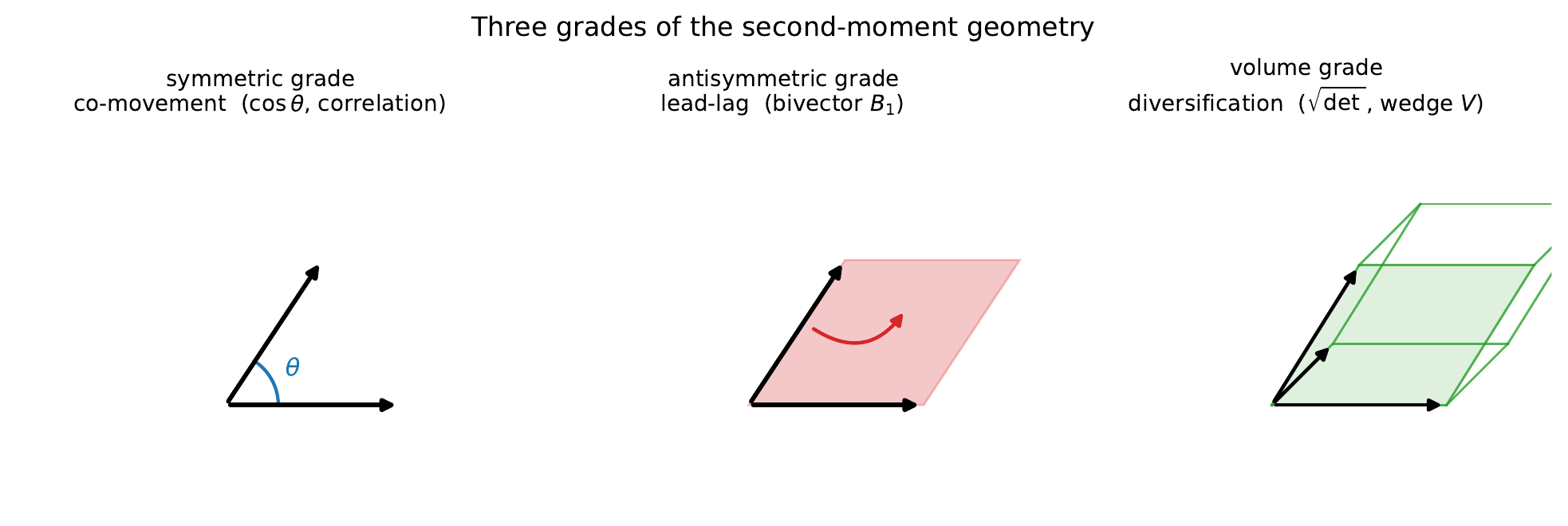
Three grades of the same return geometry: co-movement (correlation), lead-lag (the bivector) and diversification (the wedge volume).

• The symmetric grade is co-movement — plain correlation.

• The antisymmetric grade is lead-lag — the bivector B₁, which already shows growth leading defensive.

• The volume grade is diversification — the wedge volume, how much space the sectors span. It comes back later to say when.

The lead-lag grade carries a direction, but on its own it is unconditioned. It cannot tell a direct lead from a shared driver reaching two sectors at different speeds. That is what conditioning fixes.

Direction, tested properly, comes from an asymmetric question. How much variation is left in the proposed effect after you predict it from the proposed cause and the controls? For a candidate edge from today’s return iₜ to tomorrow’s return jₜ₊₁, the study computes the fractional predictive improvement:

Read it left to right. First predict tomorrow’s sector return from the controls S. Then see how much adding today’s candidate cause reduces what is still unexplained. Swap cause and effect and you get a different number. The difference between the two is the directional lead score.

In geometric terms, this control step is a rejection. Project the effect onto the space the conditioning variables explain, and keep the part orthogonal to it. In a linear setting this is ordinary residualization. Here it uses radial-basis kernel ridge regression instead of a straight-line fit, because daily returns are nonlinear and heavy-tailed. A linear control would leave nonlinear confounding behind. A polynomial control would blow up on the tails. The radial-basis rejection, with ridge regularization and coverage-based landmarks, captures nonlinear structure without letting a few extreme days take over.

Co-movement and lead-lag describe the data. Conditioning is the step that turns the lead-lag grade from a description into a test for a direct effect. The geometry is an organizing language, not a license to read cause into correlation.

The direct growth-to-defensive result disappearing does not mean nothing happens in sequence. It means the sequence sits somewhere else.

With the same one-day conditional score, the market factor clearly leads the defensive group. The defensive group’s net lead over the market is −0.020, and the block bootstrap puts the probability that defensives trail the market at 0.95. Growth looks like it leads the market by +0.020, but that one is not robust in this sample (bootstrap probability 0.72). So the observed lead-lag is a composition: growth → market → defensive, with the robust link being the market reaching defensives on a delay.

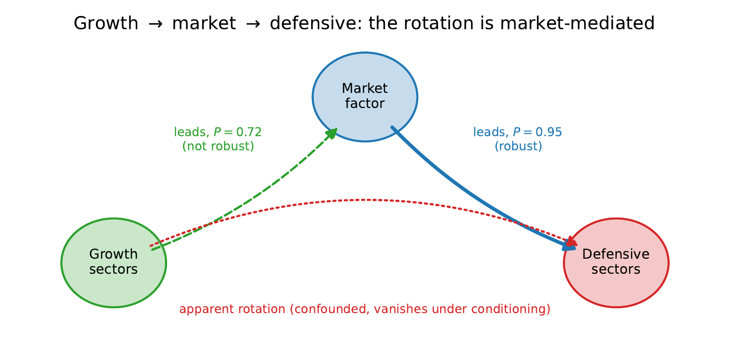
The causal structure. Growth leads the market weakly (P = 0.72, not robust), the market leads defensives (P = 0.95, robust), and the apparent direct rotation is confounded and vanishes under conditioning.

The per-sector picture is consistent. Rank all eleven sectors by their net lead over the market and every growth sector sits on the leading side, every defensive sector on the lagging side. Technology leads by the most; Consumer Staples lags by the most. The magnitudes are small, and only the defensive-lags-market side clears the bootstrap.

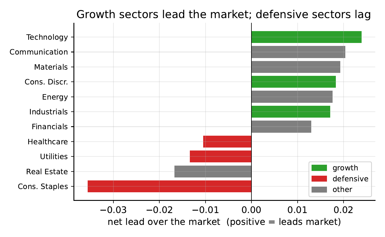
Net lead over the market for all eleven sectors. Every growth sector leads and every defensive sector lags; Technology leads by the most, Consumer Staples lags by the most.

So we have not shown a full chain from growth to market to defensives. The robust part is narrower: defensive sectors lag the market factor. The growth-to-defensive sequence we see fits growth’s higher market sensitivity plus that defensive delay. That distinction keeps the conclusion at the level the data support.

The study also asks when the apparent rotation shows up. It uses a 60-day rolling wedge volume: the square root of the determinant of the sector correlation matrix. When sectors move differently, their return vectors span a large volume. When they all move together, that shape flattens into a “risk pancake” and the volume drops toward zero. So low wedge volume marks a concentrated, low-diversification market, one where a single common factor runs the cross-section.

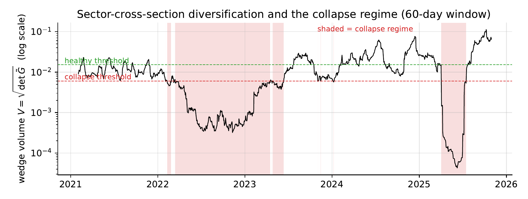
The 60-day rolling wedge volume, log scale. Low volume is the risk pancake; the shaded stretches are the collapse regime, clustered in 2022 and a short, extreme 2025 episode.

Split the sample into thirds by this volume and the result gets more specific. In the low-volume collapse regime the unconditioned gap is +0.26, with a 90% block-bootstrap interval of [0.01, 0.61]. In the healthy regime the interval is [−0.06, 0.15], which covers zero. Conditioning on the market factor removes the rotation in every regime.

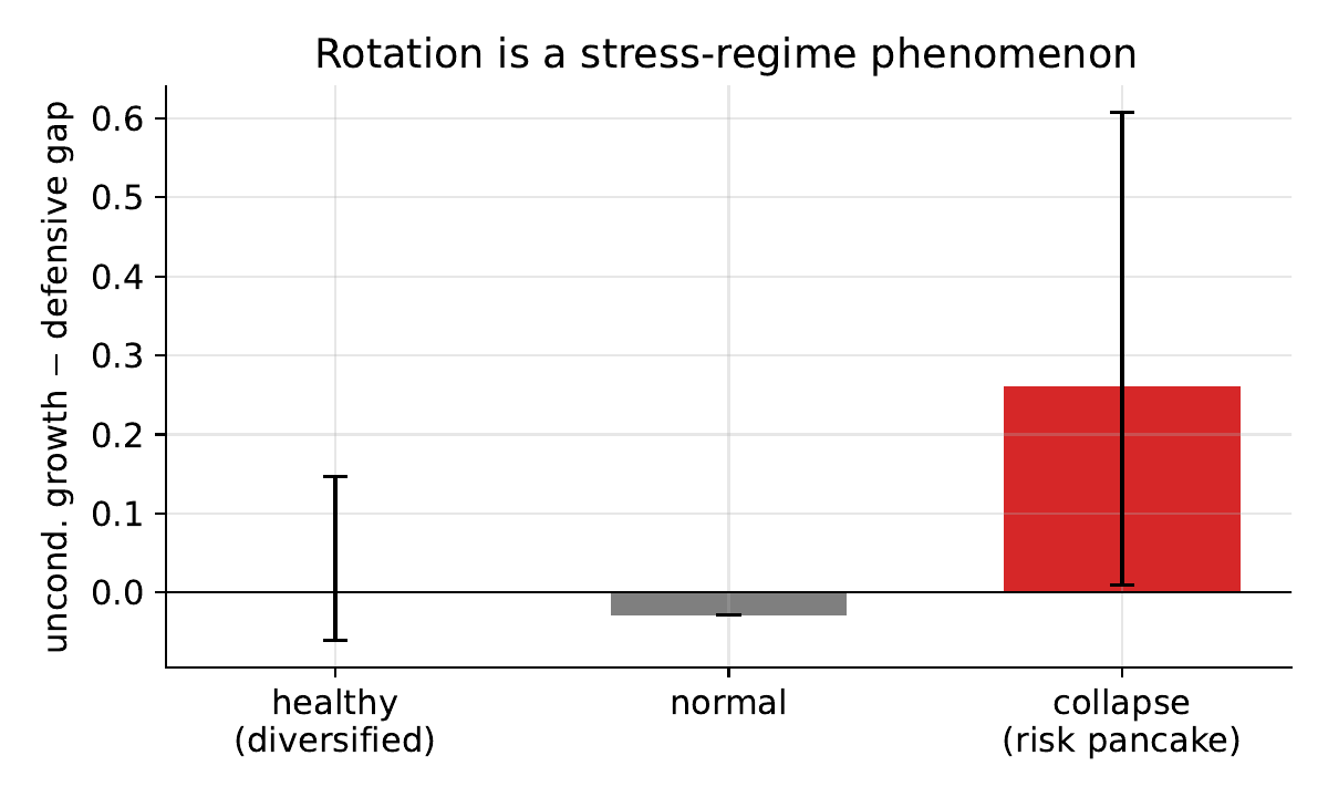
The unconditioned gap by regime. The rotation appears only in the low-volume collapse regime and is near zero when the market is healthy.

The economics fit together. Under stress, the market factor swamps the differences between sectors and reaches defensives on a lag. That lag can look like a repeatable growth-to-defensive rule. In a healthy, diversified market there is no such signal to trade.

If this holds up in longer samples and other universes, a sector-rotation overlay should be attributed and sized differently. It is not a stable, diversifying cross-sector alpha. It is closer to a market-timing exposure that only shows up once diversification has already broken down. This is the discipline of causal factor investing: separate a genuine cross-sector driver from a shared market exposure before you treat it as its own source of return. That suggests a few practical checks:

• Report the strategy’s market-factor exposure, especially in stress windows.

• Condition the signal on a market or common-factor proxy before treating it as an independent predictor.

• Use a diversification-state measure as a gate or risk input, instead of assuming the signal means the same thing in every regime.

• Test costs, turnover and out-of-sample performance separately. This study makes no performance claim.

The lesson goes beyond sector rotation. A lead-lag can be real as a description and still fail as a direct causal signal. This is not a technicality. It decides whether the signal diversifies a portfolio or just repackages an exposure you already have.

This is an observational analysis of daily sector-ETF returns over 2020–2025, a stretch that includes the 2022 drawdown and later bouts of stress. It cannot rule out a hidden common driver that the constructed market factor misses. The methodology companion has its own limits. Its residual-volume direction proxy works well for nonlinear and heteroscedastic mechanisms, but it has little power on linear-Gaussian relationships, where this signal does not identify direction.

The next steps are extension, not extrapolation. Repeat the test on longer histories, other equity universes and international markets. Compare different ways of building the common factor. Pre-specify a trading rule, then measure its out-of-sample return, turnover, drawdowns and factor exposures.

For now the conclusion is strong but narrow. The growth-to-defensive lead-lag survives several descriptive checks. It does not survive the causal one. Remove the market’s timing and the direct rotation is gone.

• Sudjianto, Setiawan and Narain (2026), Is Sector Rotation Causal? A Geometric Test of the Growth-to-Defensive Lead-Lag, SSRN 7313339).

• Sudjianto and Setiawan (2026), Causal Discovery using Geometric Algebra, SSRN 7291638.

• Code and reproductions: GA-Causal-Discovery.”