SIMD: A Practical Guide

As CPU clock speeds began reaching a plateau, hardware engineers had to find new ways to improve performance. Modern chips achieve this primarily by increasing explicit parallelism. This, however, comes at the cost of making software more complex to write.

Increases in clock speed or cache size typically improve performance without requiring any change to pre-existing code. However, this is is not the case for all hardware improvements. Fully exploiting hardware parallelism often requires software to be written in a different way.

One such form of parallelism is SIMD (Single Instruction, Multiple Data), which enables a single CPU instruction to launch multiple data operations within the same clock cycle. On modern CPUs, this typically means performing between two to sixteen operations simultaneously, potentially speeding up algorithms by the same factor.

This article shows how to effectively utilize SIMD instructions when writing software.

A new programming paradigm centered around CPU register size

The main idea of SIMD is that since a CPU instruction already has to be fetched from memory and work its way through an ever-increasingly complex CPU pipeline, that very same instruction could do more work for the fixed cost that’s already being paid to retrieve and process that instruction. This has multiple implications, even for what is otherwise scalar code. Consider the following example in C++:

A typical compiler targeting x64 would produce the following code1:

As one would expect, doing an add operation in C++ generates a floating point add instruction, however, several other things are going on here even in this simple example. The xmm0 and xmm1 registers correspond to the A and B parameters respectively. These two registers are added together and stored back into xmm0, which is the return result of this function. The ss suffix on the addss instruction stands for Scalar Single-Precision; in other words, this instruction performs one add operation using two registers each containing only one 32-bit floating point number.

What’s interesting about this particular example is that the xmm registers have space for four 32-bit floating point numbers, despite the example code above only utilizing one of the four available numbers in the register. This is because it’s possible to do four add operations at once using an addps instruction. The ps stands for Packed Single-Precision, which means that there are four 32-bit floats packed together in a single register.

To utilize all four data slots in the register, the data has to be structured in a different way than is normally done. Continuing on the example of a function that adds numbers together: if an array of four numbers packed together were passed into the function, doing four add operations at once (using an addps instruction) would actually make sense:

Instead of the compiler emitting four separate add instructions as one might expect, it uses one addps instruction instead2:

In comparison to using four separate addss instructions, executing only one addps instruction is effectively four times faster. If the array length weren’t a multiple of four or unknown at compile-time, the generated assembly would be much more complicated; this is because the instructions for loading and storing data also operate on four 128 bits of data at a time. If, for example, the array length were exactly 3, it would require the compiler to generate more instructions to deal with the non-multiple of four array lengths. If speed were critical, it would be better to pad the array length back up to 4 and not use the last array element, because while that wastes 32 bits of space, the compiler ends up generating fewer instructions.

; Adding to 4 array elements (4 instructions)
Add(float*, float):
        movups  xmm1, xmmword ptr [rdi]
        shufps  xmm0, xmm0, 0
        addps   xmm0, xmm1
        movups  xmmword ptr [rdi], xmm0
        ret
; Adding to 3 array elements (7 instructions)
Add(float*, float):
        movsd   xmm1, qword ptr [rdi]
        movaps  xmm2, xmm0
        unpcklps        xmm2, xmm0
        addps   xmm2, xmm1
        movlps  qword ptr [rdi], xmm2
        addss   xmm0, dword ptr [rdi + 8]
        movss   dword ptr [rdi + 8], xmm0
        ret

As shown above, the structure of the data in the program is just as important as what instructions are actually being used to process the data. This is often why compilers can’t automatically generate SIMD instructions for any given program; the structure of the data often makes it impossible to actually operate on four (or more) elements at a time. In the example above, doing simple add operations on an array caused the compiler to automatically generate SIMD instructions; however, real-world programs don’t often spend their time in loops that do trivial add operations on all elements in an array, and restructuring the data is sometimes not as simple as adding a few padding bytes to the end.

Retrofitting antiquated programming languages

As mentioned before, there are many situations where the compiler can’t automatically generate SIMD instructions. In the case of C and C++, this is solved by using what are known as intrinsic functions, which allow the programmer to explicitly tell the compiler which instructions to generate. What’s unfortunate about these intrinsic functions is that they lock the code to a specific CPU instruction set. This article will use the intrinsic functions for x64. To show how these intrinsic functions are used, we can start with a struct representing a three-dimensional vector:

This type is useful when adding a position and velocity together. The typical C++ approach would be to overload the plus operator to perform the addition on all the elements of both vectors:

The vector addition above is adding 3 floating point numbers that are packed together, so it would seem optimal to use SIMD instructions in this case. As mentioned before in the array example, we’d want to align the size of this type to 16 bytes (i.e. the size of four floating-point numbers) so that it matches the size of the aforementioned xmm registers.

From here, it’s possible to use intrinsic functions to explicitly tell the compiler to use SIMD instructions:

While the code above is likely to make compilers generate better instructions, it’s significantly less legible than the more straightforward add function, so the first task when reading code like this is to understand what each intrinsic function does in the context of this function. The example code above uses three intrinsic functions:

• _mm_loadu_ps: Load v3 into an xmm register

• _mm_add_ps: Add two xmm registers together

• _mm_store_ps: Store xmm register back into v3 variable

This data flow is very common when writing code with SIMD intrinsics, so to make the code directly express what we want it to do, we can write helper functions that automatically cast between the intrinsic xmm register types and the custom types we’ve defined in our program:

With these helper functions, it’s much easier to see that the addps instruction is the only important part of the overloaded plus operator:

It’s possible to apply this same logic to more than just addition, as well. One very useful resource for finding out what SIMD instructions are available on the x64 architecture is the Intel Intrinsics Guide; with this guide, one can directly search the names of intrinsic functions and find which x64 instructions they correspond to. Here are a few more examples using the v3 type:

These functions all follow a very similar pattern; this is because the math and bitwise operators in C++ correspond very closely to CPU instructions, so making wide versions of these functions is fairly straightforward. If one were to do something more complex with vectors, using SIMD instructions becomes a bit more difficult. Using the velocity example from earlier, one might want to calculate the magnitude of the velocity vector to find the distance that the object will move after adding it to the position:

The main problem, once again, is the structure of the data; there is no way to convert the length function to use SIMD instructions. The function only returns one number, which means that it will utilize non-SIMD instructions. Given that there is space in the CPU register for four numbers, it would stand to reason that it might make sense to calculate four length values instead of just one. Of course, this would also mean that this function would need four three-dimensional vectors to get the lengths from, but how is this data to be stored?

An example with ray tracing

To see how SIMD is used beyond simple four-wide packed math operations, it’s necessary to show a more complex problem; the example of this article will be a ray tracer. For those unfamiliar with ray tracing, the ray-sphere intersection algorithm is the thing that’s most relevant for this article; it’s not entirely necessary to know how it works as the important part is the type of data transformation the CPU has to make when using SIMD instructions. The reference codebase for the examples in this article can be found here.

To render an image via ray tracing, a ray has to be generated for each pixel on the screen; this ray will be used to find the closest object in the scene that corresponds to the pixel. In the following examples, we’ll use spheres for simplicity.

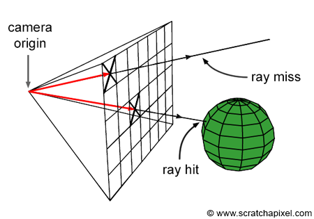
The following is an example of the basic setup work for a ray tracer; this code is meant to serve as a reference and isn’t important for understanding the underlying concepts of SIMD:

The example code above sets up a basic camera that’s hard-coded at position: 0, 0, 0. For each pixel on the screen, a ray is generated with a slightly modified direction; a ray generated for a pixel on the left of the screen will have a negative direction for the x, whereas one on the right will have a positive direction for x. To have a sphere in the scene, a data structure representing the position and radius of a sphere is needed:

To find which sphere is closest to the camera for a given pixel, it’s necessary to loop through all the spheres, find which ones intersect with the ray from that pixel position, and use the one with the smallest distance from the camera to calculate color data. A ray-sphere intersection algorithm might look something like this:

The actual specifics of this algorithm are irrelevant for the discussion of SIMD; the important part is that for every pixel on the screen, it’s looping through all spheres in the scene and finding the one that’s closest to the camera. This is to say that if there are 100 spheres in the scene, this algorithm would have to cast a ray against all 100 spheres for every pixel on the screen. Ray tracers will often have to calculate more than one ray per pixel, which will make the algorithm repeat this process of looping through all spheres several times; hence, the actual number of ray-sphere intersections multiplies to a large number fairly quickly.

For the purposes of SIMD optimization, we can focus on one line of code in particular:

The SquareRoot function takes in one number, computes the square root of it, and returns exactly one number. If we look at the corresponding assembly code, this can be seen much more clearly:

00007FF638AF138F  addss           xmm12, xmm10
00007FF638AF1394  movhlps         xmm10, xmm10
00007FF638AF1398  addss           xmm10, xmm12
00007FF638AF139D  xorps           xmm12, xmm12
00007FF638AF13A1  sqrtss          xmm12, xmm10  ; SquareRoot
00007FF638AF13A6  ucomiss         xmm12, xmm9
00007FF638AF13AA  jnbe            0x7ff638af1430 <OnRender+0x410>
00007FF638AF13B0  movss           xmm12, dword ptr [rip+0x1dbf]
00007FF638AF13B9  subss           xmm12, xmm10
00007FF638AF13BE  xorps           xmm10, xmm10
00007FF638AF13C2  sqrtss          xmm10, xmm12

The compiler generates a number of instructions that end with ss; these instructions only compute one value at a time. This includes the sqrtss instruction, which corresponds directly to the SquareRoot function. Just like with the add instruction, there is an equivalent sqrtps instruction that can compute four values at the same time. This should give a hint as to how the data should be structured to make this algorithm more parallel. The function signature of the SquareRoot function looks like this:

A SIMD version of this function that calculates four values simultaneously might look something like this:

In the original ray tracing code, these were the relevant lines of code that used the square root:

Naïvely converting this to SIMD would look something like this:

It might be a bit more clear where the actual problem lies. To correctly use the SquareRoot function in this context, we need to first obtain the radius of the sphere. If the SquareRoot function were to calculate four square roots at the same time instead of one, this part of the code would also need access to four sphere radii; thus, the data has to be structured in a way so that it can test four spheres against one ray. Reviewing the sphere struct from earlier, it looks like this:

This means that an array of four spheres would look like this in memory:

XYZR XYZR XYZR XYZR

This data structure is problematic for SIMD. In the original ray tracing code, the radius has to be multiplied by itself before passing it into the SquareRoot function. In order to use a SIMD multiply that would square four radii together, the data would have to be packed together like this:

RRRR

Naturally, if four spheres are being operated on at the same time, the sphere struct would need a way of holding four positions and radii packed together:

This may seem really counter-intuitive, especially for those who are used to thinking in the traditional object-oriented way; however, restructuring the data like this allows the ray-sphere intersection loop to have 4 times fewer iterations than it otherwise would.

SIMD: The easy way

When looking at code that uses SIMD optimizations, the aforementioned compiler intrinsics (i.e. intrinsics like _mm_add_ps) are used directly in the code. This has the following problems:

• After converting code to use the intrinsics, it loses a lot of its original semantic meaning. For example, a multiply operator would become _mm_mul_ps on x64 (or something similar for other CPU architectures).

• The code is no longer portable; code written using the x64 intrinsics will not compile for other CPUs using different instruction sets.

• Code that is written with a set of intrinsics for a newer generation of CPUs might not compile for an older generation of CPUs, even if they’re from the same manufacturer. Newer CPUs are often capable of running more advanced CPU instructions that are incompatible with older generations of CPUs

• It’s often difficult to convert scalar code to SIMD directly using intrinsics, as well as being difficult to experiment with changes.

For all these reasons, it makes sense to create some helper functions and types that make it easier to convert an algorithm to use SIMD instructions and that allow the same code to be compiled on different platforms.

The most obvious place to start is by converting the type, f32, to a four-wide type, f32x4. We can start by making a struct that holds four numbers packed together:

Suppose that we wanted to convert the following line of code to use SIMD:

After this conversion, the code should look something like this:

In C++, it’s possible to overload the + operator to use the SIMD intrinsics; adding two f32x4s together should use the _mm_add_ps intrinsic and return a new f32x4 with the result:

The same logic can be applied to all the common math operators and functions that are needed in the context of the ray tracer example:

These overloaded operators and helper functions are quite powerful in that they can be used to easily convert an otherwise scalar algorithm into one that uses SIMD:

The C++ code almost looks exactly the same in both the SIMD and non-SIMD versions of the CalculateDistance function; however, in the SIMD version, the CPU is processing four times as much data in the same number of clock cycles. Another interesting thing to note is that the resulting assembly code also looks very similar in both versions of the code:

// Scalar version
mulss xmm0, xmm0
mulss xmm1, xmm1
addss xmm0, xmm1
sqrtss xmm0, xmm0
// SIMD Version
mulps xmm0, xmm0
mulps xmm1, xmm1
addps xmm0, xmm1
sqrtps xmm0, xmm0

It’s also possible to apply this same logic to the v3 type and create a v3x4 type, but it requires a little bit more restructuring of the data. Recall that the goal is to have a v3x4 type that represents four three-dimensional vectors. The naïve way might be to create an array of four vectors in the same way as the f32x4 type, but this method is problematic since the data is stored horizontally. The horizontal instructions are typically much slower and harder for the CPU to pipeline than vertical instructions. The consequence of this is that it’s better to store the x, y, and z components of a single vector vertically as opposed to horizontally:

When stored this way, the four vectors are stored as columns, whereas the x, y, and z components are stored as rows. This data structure is known as a struct of arrays.

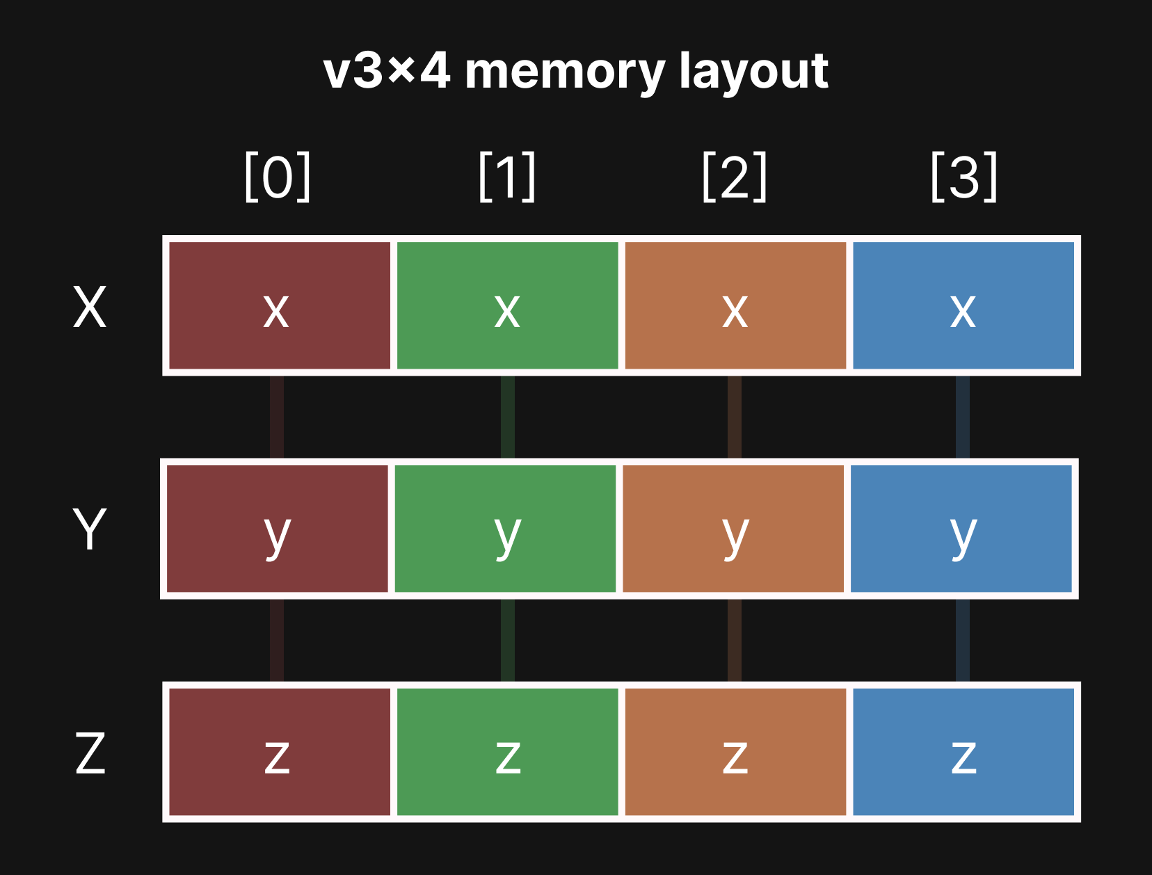
Suppose we wanted to extract out the 3rd vector from a v3x4 and store it back into a normal v3. To do that, the 3rd column (index 2) of each x, y, and z row would have to be accessed and rearranged horizontally.

One of the consequences of this data layout is that in order to add two v3x4s together, it’s necessary to use three add instructions for each row of vector components.

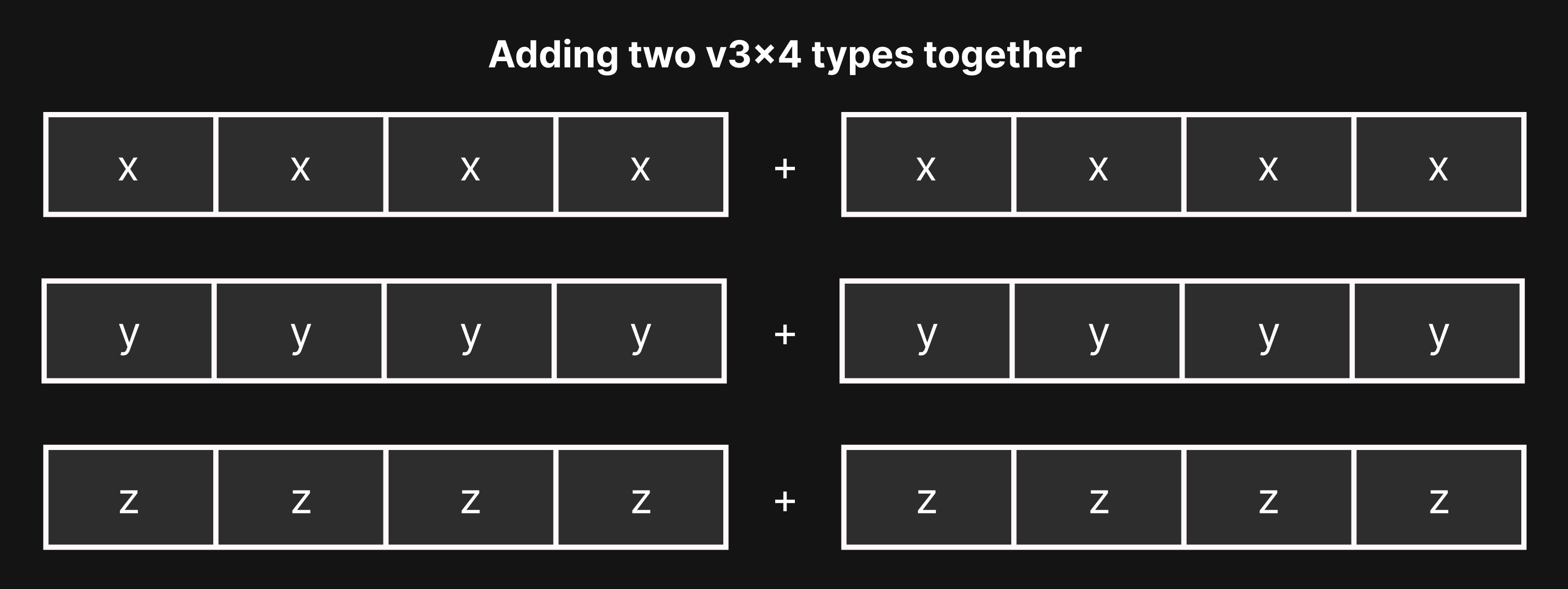
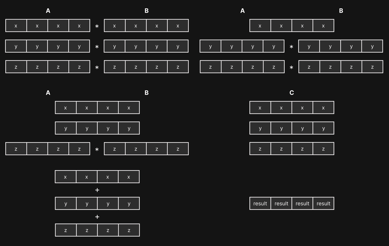
So far, this new data structure seems like much more hassle than it’s worth. Having the vectors stored vertically makes accessing each individual vector more cumbersome, and all the common math operators require using three CPU instructions instead of one. Both of these things are not actual problems in practice. First, when processing large amounts of data in parallel, it’s not necessary to access each of the four vectors individually; instead, the data will be processed without depending on the result of a neighboring column vector. Second, whilst it does require three CPU instructions to do a basic vector add or multiply, this usually won’t amount to a huge performance difference, given that modern CPUs can process non-dependent instructions in parallel. These math operations will often be overlapped with each other. Finally, this data structure allows us to easily convert other vector operations to use SIMD instructions that would otherwise be impossible to convert. As an example, here is the vector dot product as it is normally written:

This can also be written in a way to more explicitly use a SIMD multiply instruction:

The problem with this code is that the data is laid out horizontally. Instead of executing many things in parallel, the result has to be combined back into one floating point number.

Using the newly created f32x4 type, it’s possible to convert the dot product function to use SIMD and calculate four results at the same time:

While this code is superficially similar, the actual transformation of data is vastly different. All the operations are done vertically, which allows four independent results to be computed in parallel.

With these helper types, it becomes fairly straightforward to accelerate a number of algorithms with SIMD. Coming back to the ray tracer example, this introduces a problem with storing the data. In the original code, the spheres are laid out in an array like this:

With the SIMD types, the sphere array would look something like this:

Laying out spheres in code like this becomes rather cumbersome. This is also compounded by the fact that keeping the original scalar version of the code might be desirable for benchmarking, debugging, and being able to compile on platforms that don’t support SIMD instructions. In C++, it’s possible to use constexpr to convert the scalar data layout to a SIMD data layout at compile-time.

SIMD if statements

There's another challenge when converting the rest of the ray-sphere intersection code to use SIMD instructions: We can't use if statements in the same way as they are used in regular code. The purpose of the if statement in the original ray tracing code is to skip over unnecessary computations if the ray and sphere don’t intersect.

In traditional, scalar code, comparing two floating point numbers would give a true or false answer; however, when using the f32x4 type, a comparison gives four results at the same time. The only time that it’s possible to use an if statement to skip over a section of code that uses SIMD is if all comparison results are the same. In the example code above, this would happen if a ray misses all four spheres that it’s being compared against. If the comparison result is different for each column in the SIMD lane, things become a bit more complex. This would happen when a ray misses two spheres and intersects with two other spheres. A simple if statement is no longer sufficient; it only makes sense when none or all of the comparison results are true.

Overloading the comparison operators for the f32x4 type is fairly straightforward because they correlate one-to-one with x64 CPU instructions.

What’s interesting to note about the SIMD comparison instructions is that for each SIMD column, if the result is false, it fills the column entirely with zero bits, whereas if the result is true, it fills the column entirely with one bits; therefore it’s easy to check if all four comparisons are false by checking if the entire register is set to zero.

On x64, there is a movemask instruction, which takes the most significant bit of each SIMD column and collapses them into one 32-bit number ranging from zero to fifteen. Each bit of the result of the movemask instruction corresponds to the result of the comparison instruction. This is to say that if the result of the movemask instruction has the third bit set to one (value of 0x4) and all other bits set to zero, it would mean that the third SIMD comparison returned true and the other three results were false.

If all four comparisons fail, the result of the movemask instruction is going to be zero. In the case of the ray tracer, this would be used for skipping unnecessary calculations if the ray doesn’t intersect with any of the four spheres that are being tested.

Of course, things won’t always be this easy; sometimes, memory has to be moved based on a certain condition being true. A ray tracer has to find the sphere with the distance that’s closest to the camera, which means it has to move memory based on the result of a less-than comparison. Having the comparison instructions return all ones or all zeroes is quite helpful in this context because bitwise AND instructions can be used to mask away undesired results.

Blending results together like this is such a common operation that Intel introduced an instruction specifically for this purpose:

This conditional move helper function opens up a lot of possibilities for using SIMD instructions since it’s possible to use conditional code with a single stream of instructions.

This is where some of the complexity of SIMD comes from. The scalar version of an algorithm may be faster than the equivalent SIMD version due to it being able to more properly take advantage of branching. This is also why sometimes converting an algorithm to use SIMD won’t necessarily make it four times faster; there’s usually some form of overhead when an algorithm requires lots of branching or data to be pieced back together. Using the ConditionalMove helper function above as an example: an extra instruction, blendvps, must be used to mask away undesired results; furthermore, even if three of the four conditions are false, the CPU still has to execute all of the instructions that a scalar version would be able to skip. Keeping a scalar version around is useful to make sure that there is an actual performance benefit from using SIMD instructions.

The final part of the ray-sphere intersection test loop has this conditional code:

Because all code past the if statement only happens if certain conditions are true, all places where values are stored based on this condition have to be wrapped in the ConditionalMove helper function when using SIMD.

Another place where knowledge of how the SIMD comparison instructions work is when normalizing a vector. Normalizing a vector requires calculating the length of a vector and dividing all its components by that length; the resulting vector has a length of one. This can be done using all the information already presented so far:

A problem that one might run into when normalizing a vector is that it’s possible to pass in a vector of length zero into this function. This would cause the function to divide by zero and output invalid values into the register. In a typical normalize function, this would be checked with an if statement, however, with SIMD, it’s necessary to use bitwise operations to mask out values that have been divided by zero.

Conglomerating four results back into one

Coming back to the original ray tracing example in its entirety, the code should look something like this after swapping out all f32s and v3s with their four-wide counterparts:

The code above would, in the best case, be four times faster, since the for loop is iterating over four spheres at a time instead of just one. If there were 100 spheres to process, the SIMD-optimized loop would only iterate 25 times. The one remaining problem is that because four spheres are being processed in parallel, we end up with four different results at the end of the loop.

The correct color value should come from the sphere that is closest to the camera. The problem is that this information is stored in the MinT variable, which is an f32x4 that contains four separate values. This means that in order to get the correct color value, it’s necessary to find the smallest value in MinT, get its index, and use that index extract the correct column out of Color. The most naïve way to find a minimum value out of an f32x4 would be to simply iterate over all four values and find which one is the smallest.

The above function implementation, while easy to understand, is not likely to generate good code; a more optimized version would look something like this:

Recall that with the SIMD ray tracer, there are four computed color values after the ray-sphere intersection loop is done processing. These color values are also stored vertically, so once the correct color value is known, it has to be reassembled back to a normal color value that can be output to the screen. The correct color value has the same index as the lowest t-value (i.e. distance from the camera and/or ray origin), which is obtained by using the newly created HorizontalMinIndex function.

After these changes, this barebones ray tracer should produce the same image, except a little bit faster than before.

Another important thing to note is that this way of indexing into the sphere colors also handles cases where the number of spheres is not an exact multiple of four. If a fifth sphere were added to the scene, the radii of the other three spheres in the SIMD sphere group could simply be set to zero, which causes them to be ignored.

Setting the radius of a sphere to zero guarantees that the ray won’t intersect with it. Because the conditional move functions already prevent the resulting color and min t-value from being written to when a ray-sphere intersection fails, the code can gracefully handle any sphere with a radius of zero; this is very useful when the number of spheres is not an exact multiple of four.

It’s possible to take these techniques and apply them to a more fully-fledged ray tracer. The advantage now is that with SIMD, the ray tracer can process four spheres simultaneously. When the scene only has four spheres in it, the SIMD version is likely to be faster, however, it won’t be four times faster; the SIMD version has some extra overhead due to the way branches execute and the reassembly of data using the horizontal min. The good news is that as the number of spheres increases, the proportion of overhead to the total amount of work being done will decrease, which causes the SIMD version to get much closer to the 4x speed increase one would expect. The only way to know for sure is to benchmark the code; the reference codebase is provided here for this purpose.

The next steps…

This article focused on how to take a real-world program and optimize it in the context of an x64 CPU with the SSE extensions, however, this is only the beginning of a journey into learning SIMD. Most newer x64 CPUs support an extension called AVX2, which allows eight-wide 32-bit operations, in addition to several other enhancements to the instruction set. The vast majority of other instruction sets that are relevant today also support the types of SIMD operations talked about in this article, including ARM, RISC-V, PowerPC, WebAssembly, and so forth.

The race to build the fastest CPUs for the lowest cost never ceases, and SIMD instructions seem to be a part of that for the foreseeable future. If nothing else, it’s a good way to challenge one’s skills as a programmer and think outside the normal programming paradigm. Hopefully, this article makes the process of learning how to optimize programs using SIMD just a little bit easier.

- Caden Parker