
When Recursion + MIT co-released Boltz-2 with its open-sourced structure and affinity predictor, most people were excited about how it could make drug design cycles faster and better. But I was thinking bigger! Arguably, a cell’s function is dictated by billions of interactions between proteins, RNA, DNA and small molecules, so why not try to simulate them all 🤯! This is finally possible with the newest generation of accurate and scalable models.
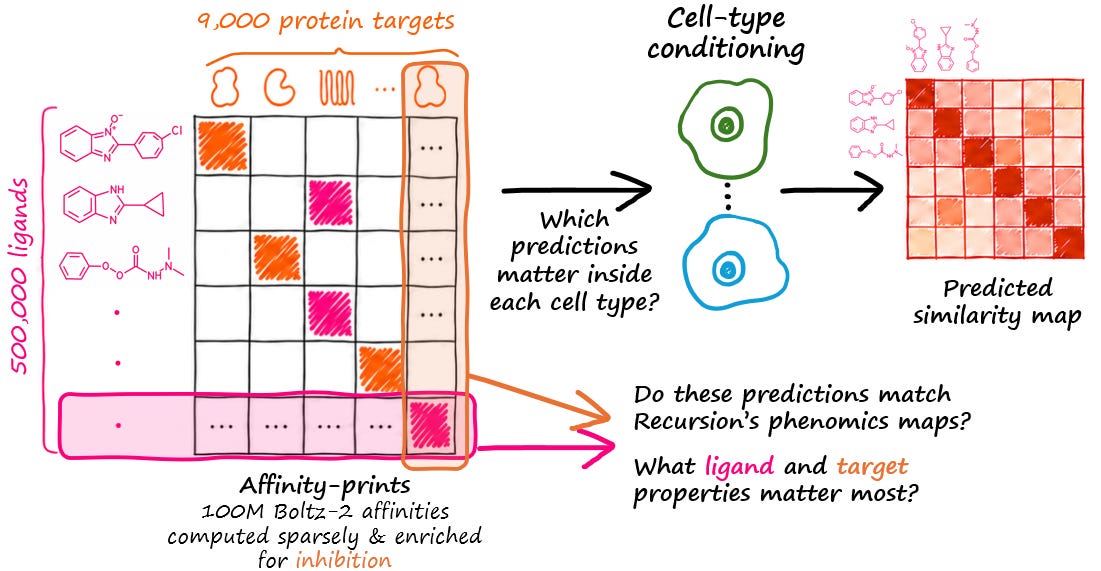
So for the past 12 months, I have used pre-emptible GPUs to run AlphaFold Multimer protein-protein co-folding, or Boltz-2 protein-ligand co-folding with affinity predictions, leading to an enormous dataset of 100 million co-foldings, spread across 9,000 unique targets and 500k ligands. I call this dataset affinity-prints.
Running co-folding 100 million times was the easy part. The hard part was figuring out which of these predicted interactions actually matter inside a cell.
And this is where Recursion’s large-scale phenomics datasets can be uniquely leveraged: to study the relationships between the affinity-prints and our cell-based assay data. More importantly, Recursion’s large phenomics maps allow me to identify a vast amount of likely protein-protein or protein-ligand interactions, enabling me to sparsely screen such a large space more efficiently.
And what I found was amazing! Here are some key insights:
I built the smallest Virtual Cell with as few as 6 parameters, showing that, by coupling dense affinity-prints with Recursion’s biological maps, we can estimate phenomics similarity maps. But this wouldn’t be possible without our proprietary datasets of gene expression and of gene-gene relationships.
I created a simple data-driven ligand score (Lig2Cell) that assesses how effective a ligand will be inside the cell, and showed significant hit-enrichment compared to traditional Lipinski rules or QED metrics.
I studied the factors that make a protein more druggable and amenable to co-folding, and found that protein class doesn’t matter much, the most important factors are the cell components (where a protein is located), the protein function (what the protein does), and the lipid coverage.
In summary, scaling up inference compute for co-folding to millions of interactions can create a new data layer, but Recursion’s biological maps are what make it useful, helping build Virtual Cells, and analyse the failure modes of the model.
Everything is just a proof of concept for now, but the ideas are there. Hopefully it helps kickstart an era of co-folding aware Virtual Cell models, and phenotypically aware co-folding. There will be many bumps along the way, but I am definitely excited by a future where co-folding and biological data can complement each other 🚀. Especially, given that affinity just got 20x faster with Nesso-1, we could compute billions of interactions.
Affinity-prints. Briefly, the affinity-prints are a sparse matrix consisting of a small molecule as rows, protein target as columns, and the predicted binary affinity in each cell. For each target, I would launch a low-priority pre-emptible job that runs co-folding and affinity computations. With Recursion having its own on-prem super-computer, this meant that the effective inference cost was very low.
Each protein target is segmented to only keep non-disordered and continuous segments of the sequence. Some targets get separated into two or more segments. Then, we run the affinity on each segment separately, and compute the max-pooling over each segment. For most targets, there is a single segment, but ~10% of targets had 2 or 3 segments.
For the current blogpost, I only consider the binary affinity of the Boltz-2 model, discarding any structural data, confidence, or affinity regression. This choice was made to make the analysis simpler since the binary affinity summarizes well the interaction with a single number, while also generalizing much better than the regression value on a vast chemical space.
Protein-protein interactions (PPI). For the protein-protein interactions, we want to consider all pairwise interactions between the 20k proteins from the human genome. However, that number is too large so we leverage our phenomics geneKO map to find the 1% most likely interactions, and assess them with AlphaFold-multimer. The phenomics geneKO map is built by running a gene knockout experiment for each human gene in a cellular microscopy assay, then embeds them and computes their pairwise similarities. Hence, we consider that two proteins are likely to interact when they have a similar microscopy-visible effect on the cell. You can learn more about our open-sourced RxRx3 dataset, and how these maps can be used to recover biological knowledge.
Similarity maps. I will often use the terminology “maps” to refer to a matrix of pairwise similarities between phenomics perturbations. In the blogpost, these similarities are measured for compound-compound pairs, compound-gene pairs, or gene-gene pairs.
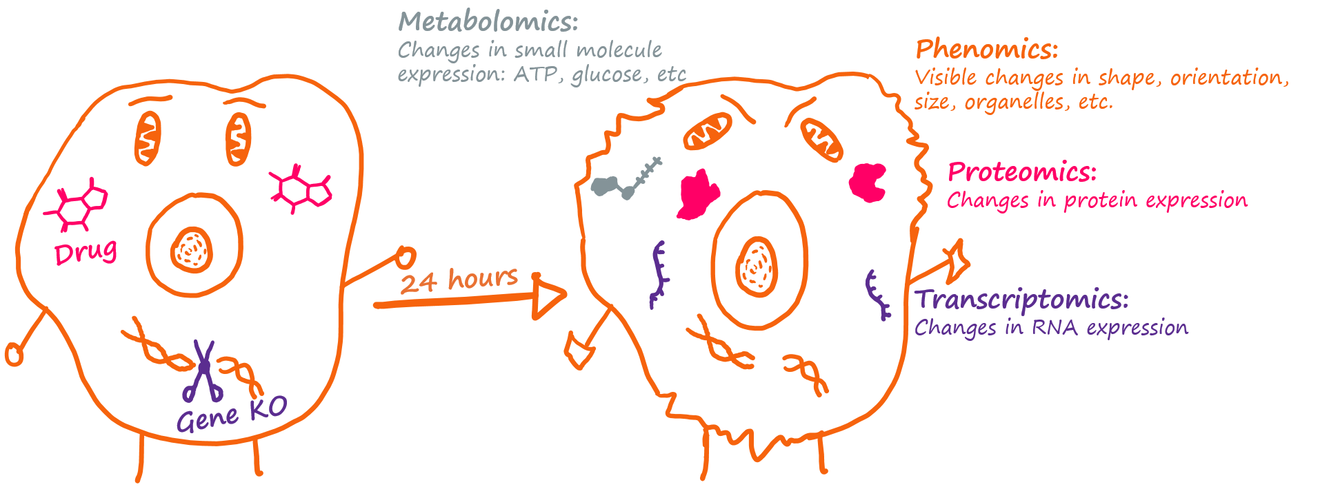
Omics. Most of the blogpost focuses on phenomics data, with some transcriptomics used in the Virtual Cell model. These data are often collected by measuring either the visible changes to a cell under a microscope (phenomics) or the change in gene expression (transcriptomics), after applying a perturbation such as adding a small molecule or knocking out a gene.
Ok, enough methods, let’s go to the results!
In this section: I will show you how I built the smallest Virtual Cell with only 6 parameters. This required taking millions of affinity predictions to build fingerprints. Then, with the help of biological insight from Recursion’s maps, I was able to filter, pool, and project them into a representation of the compound’s effect in a cell.
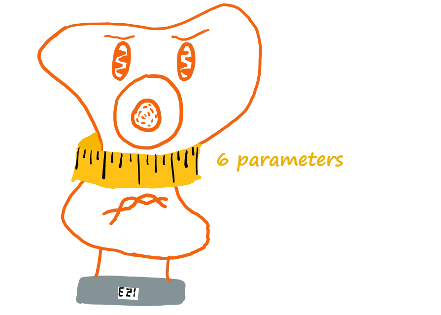
I’ll get a lot of flak for calling it a Virtual Cell, but think of it as a toy example, a proof-of-concept that we can calibrate affinity signatures to omics maps in an interpretable way. Check out this substack to learn more about Virtual Cells, and our positioning paper.
This is a completely different direction than typical Virtual Cell research: the field talks mostly about a top-down approach that trains ultra-large generative/predictive models to accurately predict the effect that a compound or geneKO has on transcriptomics or phenomics assays. Instead, we are looking for a bottom-up approach, one that builds the set of all possible interactions to determine the outcome.
How it works: In the figure below, you can see the 6 trainable parameters in orange. As input, I have computed the Boltz-2 binary affinity predictions for 6,000 ligands against 4,000 proteins (or 5,000 segments), and used a PPI map containing 4M AlphaFold-Multimer predictions, for a total of 34M co-foldings (6,000 * 5,000 + 4M). In the diagram below, we can see the architecture and better grasp how the data and parameters fit together.
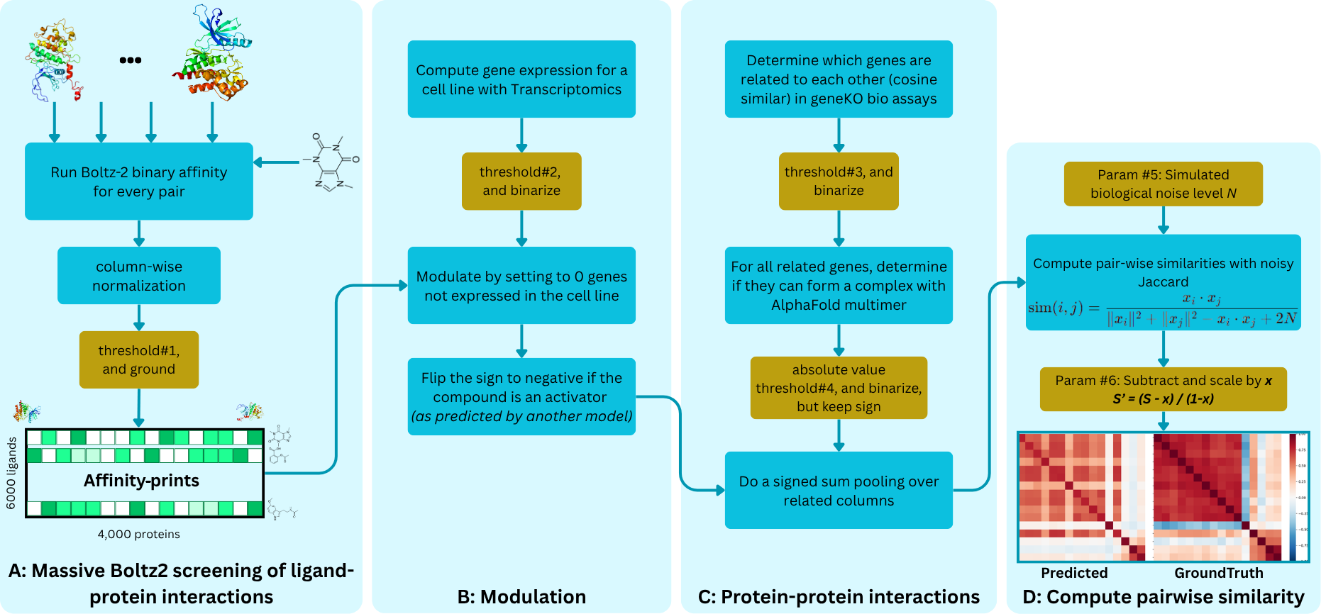
Essentially, the parameters are simply thresholds in between to remove the noise coming from non-binders. The algorithmic steps are:
Generate the affinity-prints, a dense matrix of binary affinity predictions for protein-ligand interactions over thousands of proteins, and threshold. This gives a sparse vector that annotates only the strong interactions.
Modulate by expressed genes in a cell line (with Transcriptomics). This allows us to adapt the output to each cell-type by ignoring or amplifying the interaction vector based on whether a gene is strongly or weakly expressed within a cell.
Flip the sign if it’s an activator (I have a pretty bad MLP+ESM for that), since activators will tend to have an opposite effect than inhibitors or GeneKO.
Pool together interacting proteins using our PPI network, based on our GeneKO similarity map and AlphaFold-Multimer simulations. So, if a compound inhibits protein A, and A’s inhibition phenotype is correlated with protein B, then it also has an inhibition phenotype on B.
Compute noisy pairwise similarity with modified Jaccard. This mimics the dampening of similarity maps in biological experiments when the signal-to-noise ratio is often weak.
Re-scale by a factor to make the map look nice.
How Recursion’s data come into play. In this simple model, it is important to remember that a lot of inductive biases come from our biological data, so the model doesn’t learn everything from scratch. First, it uses the transcriptomics maps to modulate the genes. Second, it uses the phenomics maps to infer both the intensity and sign of gene-gene relationships. Third, it lets us model protein-protein interactions efficiently.
Despite having only 6 parameters, the model reaches an average AUROC of 71% per cell line when recalling similarities above 0.4, and 76% above 0.6. I fitted the parameters on phenomics similarity maps from 11 blinded cell lines and 246 known compounds, representing 665k matrix elements. Quite a difficult task for 6 parameters… See the GIF below, where each snapshot is a different cell line.
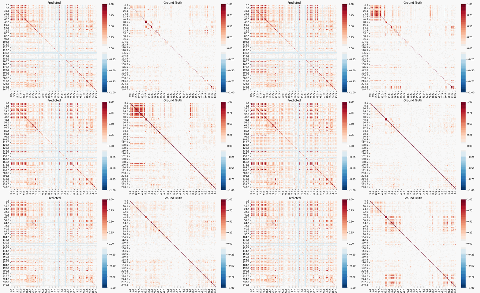
Note: These are known compounds. This means that Boltz-2 is likely to have trained on them, and that they are usually selective and drug-like, making the task easier. However, given how the task itself is widely different from training, I believe that the generalization is still impressive. Also, most of the public data Virtual Cell benchmarks are also biased towards known compounds.
Even more exciting is that the model is not too sensitive to hyper-parameters, as we can see on the histogram below. This showcases the strong biological expressivity of the affinity-prints, but also shows that biologically grounding them is important.
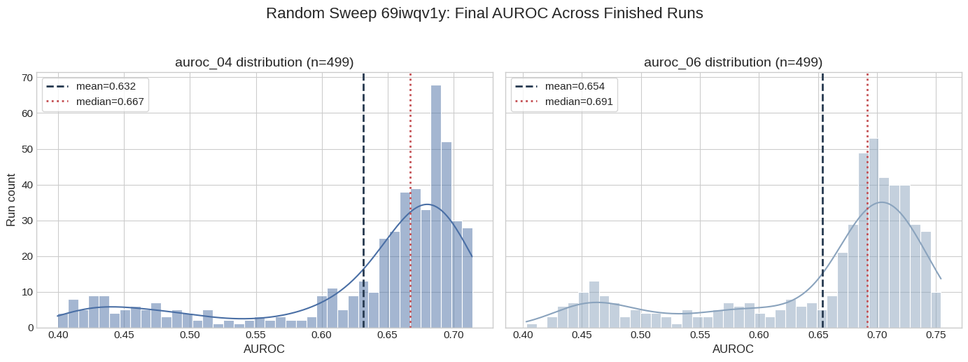
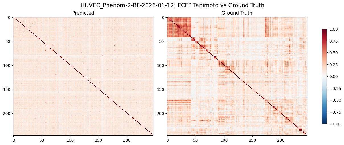
With ECFP similarity, the AUROC was much lower at 63% and 64% respectively, worse than the median of random parameters; and it only captures a few highly similar compounds. You can check the ECFP results, and some ablation studies, in the appendix.
Essentially, every time I added a new complexity in the design, inspired by our biological data, I was able to improve the results further. It is clear that the path forward is not simply more co-folding computation, but stronger grounding into cell biology, and this can only be achieved by leveraging large-scale datasets like the ones available at Recursion.
Despite its simplicity, this is the first attempt at a framework that maps from a chemistry binding model to a biologically relevant model with only some calibration. Computing pairwise similarity helps eliminate a lot of the noise from Omics and makes the task easier. The method can be extended to toxicity panels, neurological effects, anti-microbial discovery, etc.
But the affinity-prints require massive inference-time compute. If only there was a faster alternative to Boltz-2… Oh wait! Valence and Recursion just released a 20x faster affinity model, check out Nesso-1.
These are all cool preliminary results, but they are quite limited and biased towards known compounds with well-defined modes of action. Indeed, the model implies that the proteome signature of a compound, its affinity-prints, directly corresponds to its phenotypic biological signature. But cells are resilient, compounds can have non-selective behaviour, and affinity predictions might not always generalize.
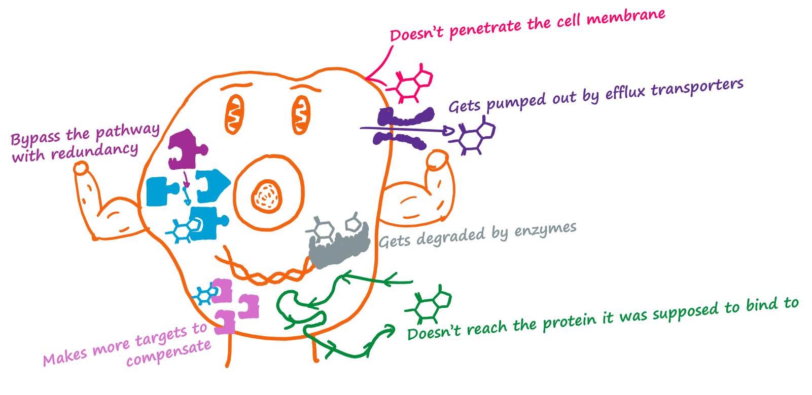
Cells are resilient, and it’s great! We don’t want any external chemistry to do whatever it wants to our body. But when it’s time to fix our body from diseases, this resilience plays against us. Let’s look at a shortlist of resiliency mechanisms from the cell that can stop your compound from being effective.
Cell membrane: The very first barrier, an oily bubble that stops any compound unless they have the right balance between water and fat solubility, or go through a specialized route in, like a transporter, channel, or cellular uptake mechanism.
Efflux transporters: Got through the barrier? The police can still escort the compounds outside with dedicated pump proteins such as efflux transporters.
Enzymatic degradation: Being expelled is the good way to go. Instead, some compounds can be broken down by intracellular enzymes and metabolized into inactive fragments before they ever reach their target.
Target inaccessibility: Maybe the compound is simply lost and cannot find its target since it’s in a hard-to-access cell component
Natural ligands: Perhaps the target doesn’t care about the compound since it has a strong natural ligand that outcompetes any novel compound.
Pathway redundancy: Even when the compound hits its target perfectly, the cell may simply activate a parallel or compensatory pathway to maintain its normal function.
Target amplification / upregulation: Or maybe the cell will just make more of the protein to maintain its function.
Sometimes, it is not the cell that prevents a ligand from achieving its goal within the cell. It could be that the ligand might not be selective for the target of interest, or to the function that we try to inhibit/activate. For example, the ligand might hit other proteins with higher affinity, or weakly hit other proteins that have a stronger phenomics effect, like toxicity. Or perhaps the ligand inhibits the target in a way that differs from the desired GeneKO or functional inhibition.
In the following section, I will address the key properties of a ligand that enable it to achieve its desired biological effect.
In the phenomics map, there are many genes that are correlated because they either share a complex or a pathway. For example, it could happen that gene A and gene B are strongly correlated for all ligands, even if each ligand only ever binds to either A or B.
My toy Virtual Cell takes this into account, but the rest of the blogpost does not, which means that there’s an added source of noise.
Another obvious failure mode is that Boltz-2 doesn’t always generalize. In this study, I looked at 9k unique proteins and 500k unique compounds, a space way larger than the training set.
In this study, I will try to assess the properties of ligands and targets where Boltz-2 doesn’t generalize, but it is unfortunately very difficult to decouple whether the cause is due to cell resilience, to compound non-selectivity, or to errors in the affinity predictions.
Also, a large part of the study is done by measuring the phenomics similarity between a geneKO and a ligand perturbation, which is correlated but not identical to the affinity predicted by the model. I will circle back on that later.
We learned that many affinity-to-phenotype failures are not about binding, but about undesired mechanisms within the cell.
In this section: I explore which ligand-level properties improve the correlation between predicted binary affinity and phenotype-based biological assays. This made me re-discover some of the most important guidelines of drug design (e.g. Lipinski’s rule of 5). Finally, I design a simple Lig2Cell score that shows a much stronger hit-enrichment rate compared to the traditional rules.
As you have seen earlier, Recursion likes to build maps of biology. I use one generated with an older deep learning model from 2022, containing ~7k proteins with a strong GeneKO signal and ~500k ligands. For each target, the top 1% of ligand–GeneKO pairs by absolute cosine similarity are marked as TRUE. Why not use a newer map built with Phenom-2? Well, I was in a hurry before going on leave, so I cut a few corners 😅.
This is where Recursion’s massive in-vitro datasets become the key: they let us learn which compounds are most likely to translate from predicted binding into a real cellular effect.
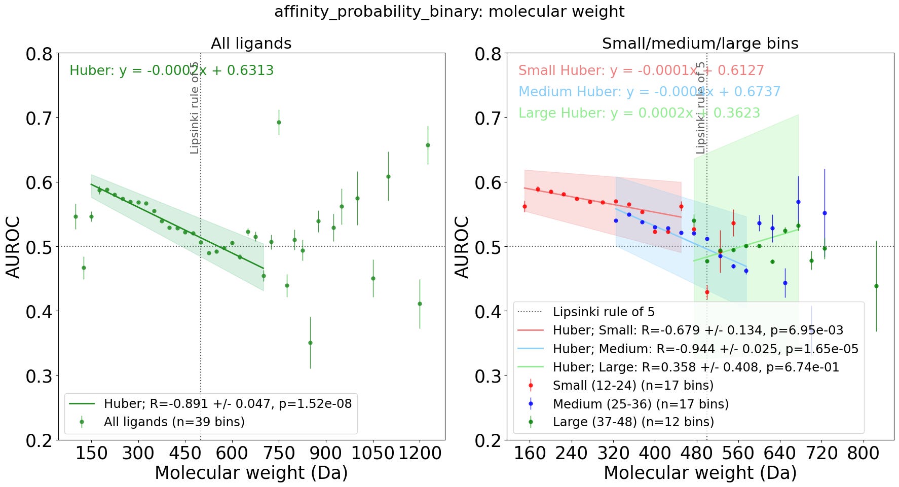
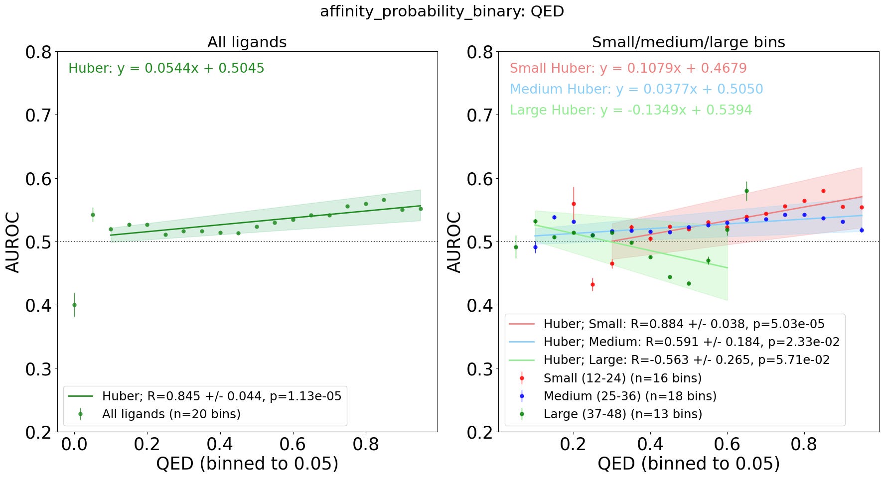
I compute Boltz-2 binary affinity for most TRUE pairs and 0.5% of randomly selected FALSE pairs, then measure how well these predictions agree with the phenomics map. For each molecular property, I bin ligands and compute the AUROC between binary affinity predictions and the phenomics map. For example, I group all ligands with 20 heavy atoms, or with cLogP between 2.5 and 2.6. A higher AUROC means either that binary affinity generalizes better or that the ligand is more likely to produce its intended cellular effect.
Overall, this gives a sparse affinity-print with more than 35M interactions. Despite the confounding factors, I argue that the results mostly reflect the assay-to-cell translation because the emerging rules align remarkably well with traditional drug-design principles such as Lipinski and Veber.
Thanks to the sheer scale of data, we can go further and decouple the correlated effects between molecular weight, cLogP, ring count, and H-bond donors. By separating ligands according to heavy-atom count, we can derive a new set of empirical rules. Unlike Lipinski and Veber, which were derived from human and rat data, respectively, our rules come from cell assays.
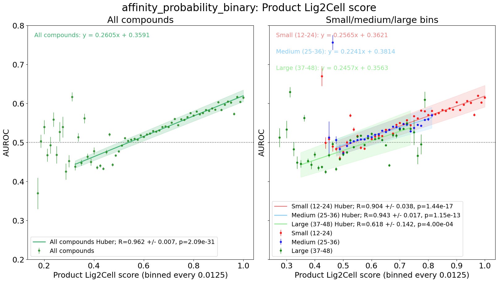
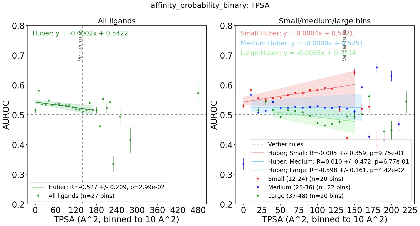
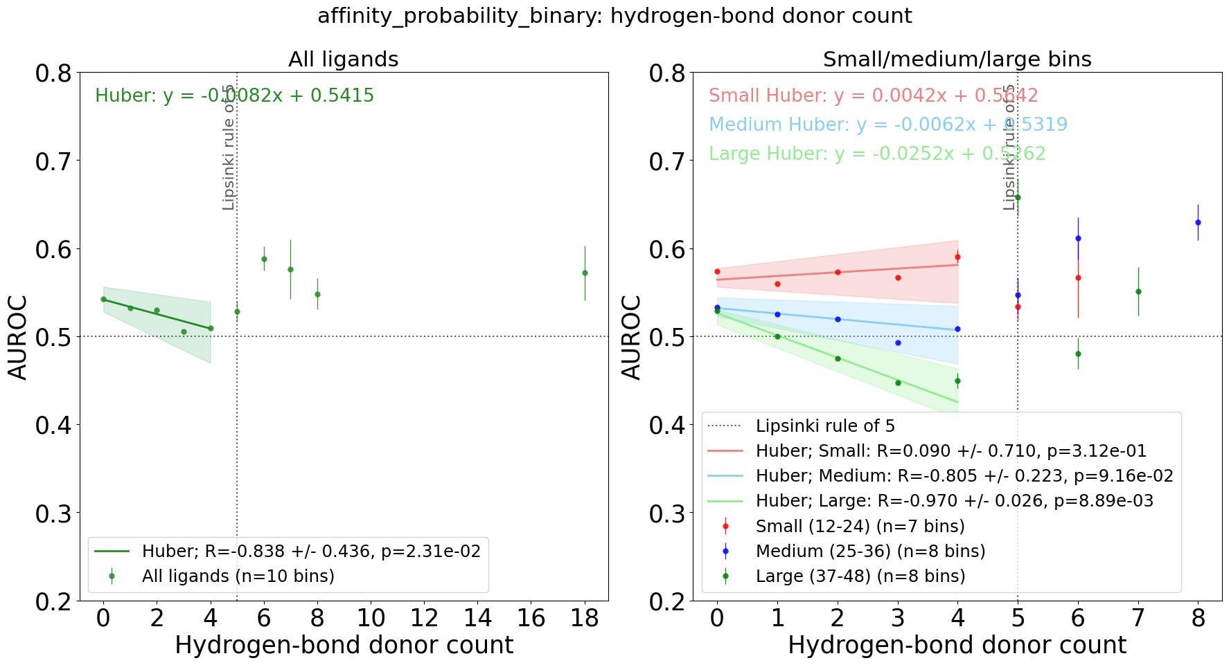
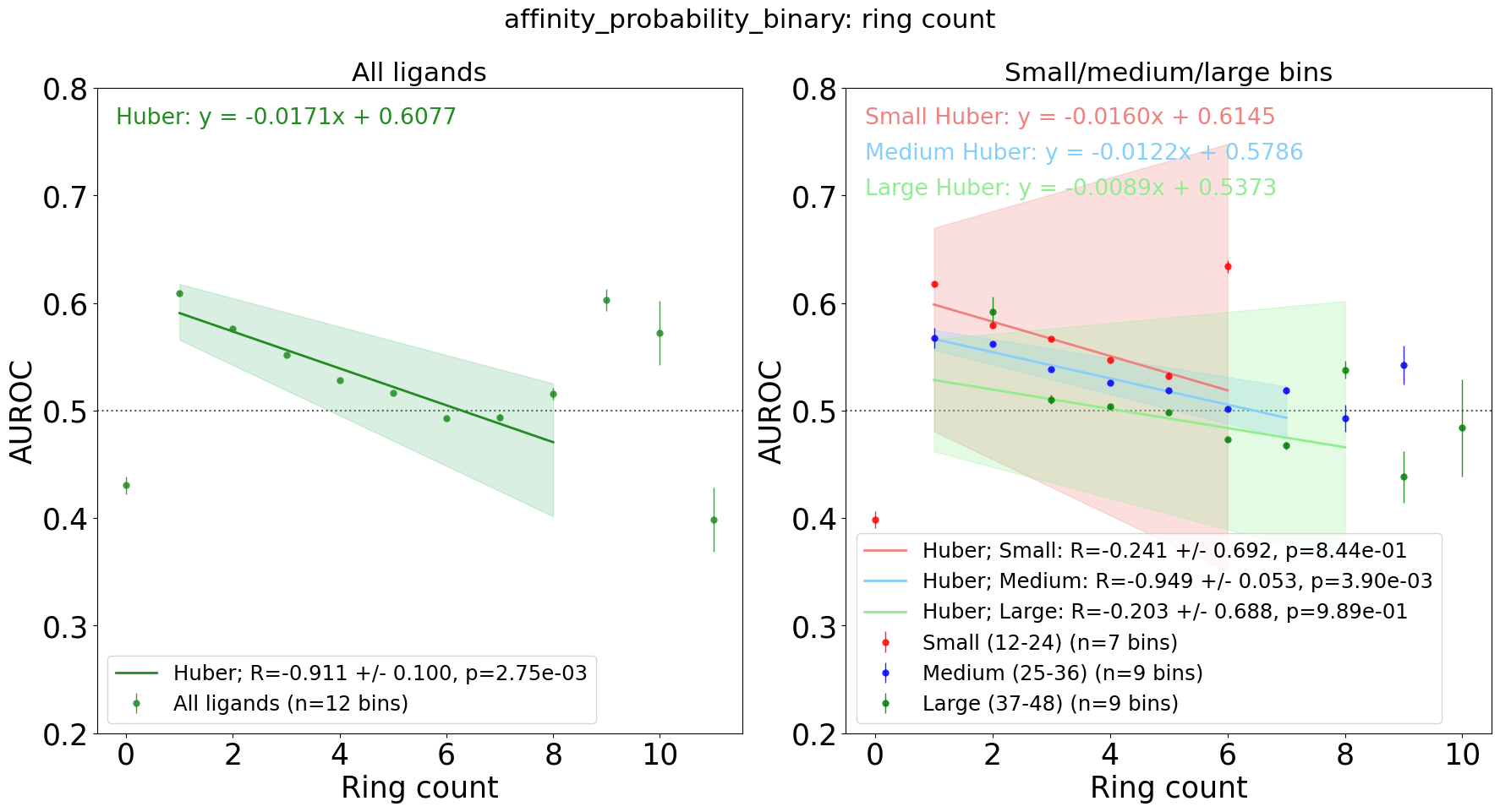
In the table below, I compare these rules across three empirically selected groups: Small, with 12-24 heavy atoms; Medium, with 25-36; and Large, with 37-48. Error bars use 20-fold bootstrapping. Trendlines use Huber regression, excluding points with a bootstrap deviation above 0.02 between the 10th and 90th percentiles.
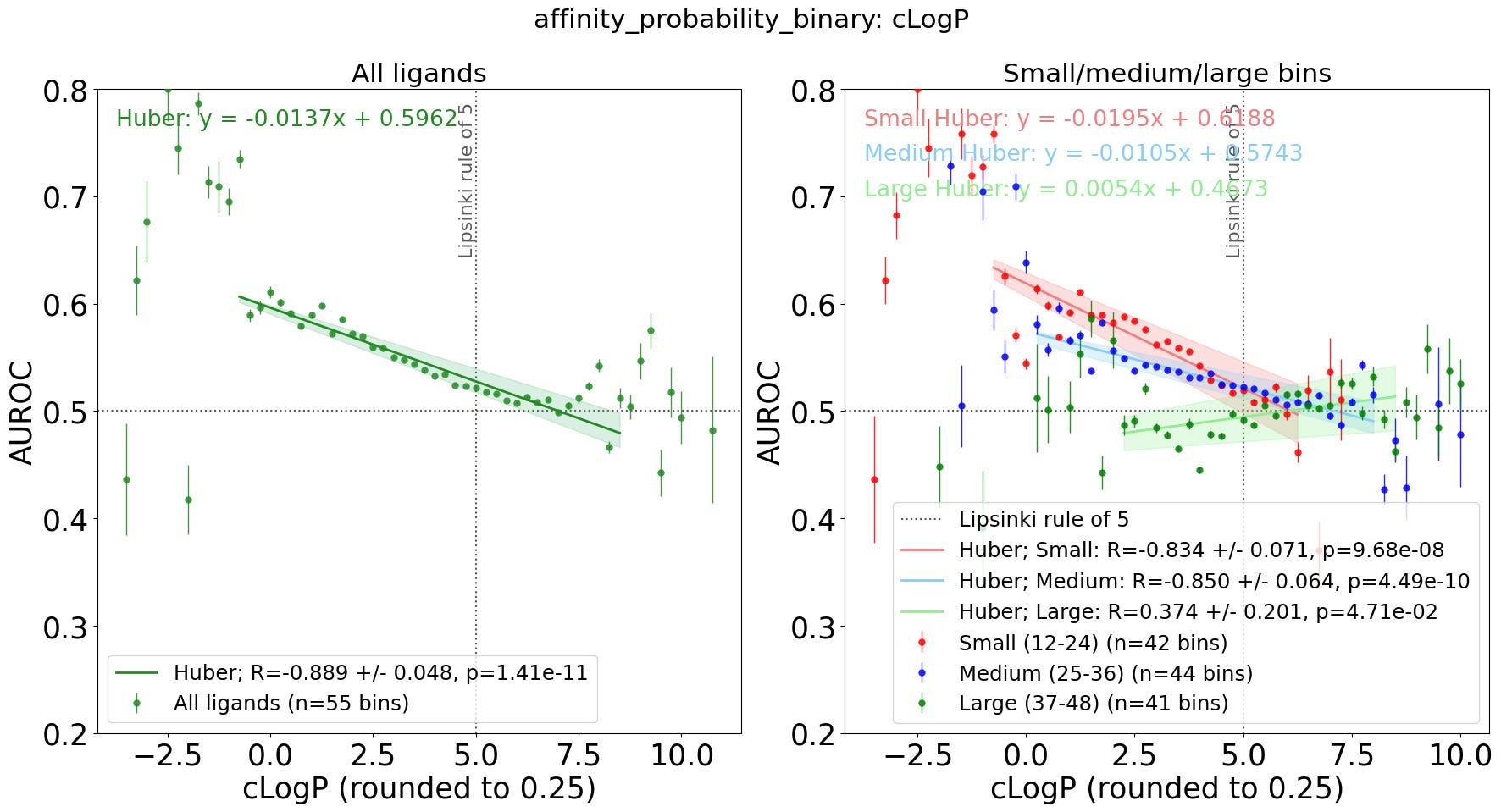
I tried this with 14 properties, so I moved it to the appendix. In summary, the most important properties are the molecular weight, the cLogP, the ring count, the aromatic ring count, and the number of hydrogen bond donors. Other properties are either weakly correlated like QED, or suffer from Simpson’s paradox when controlling for molecular size, like TPSA or number of rotatable bonds.
Taking the analysis from all 14 properties, I decided to create a new Lig2Cell score that combines the heuristics that we found from reading the plots. Each compound starts with a score of 1, and gets penalties p_i if it’s too heavy, has too many hydrogen bond donors, etc. Then, I multiply all the penalties (1-p_i) to get the final score.
I ran an evolutionary optimization of the heuristics with Shinka Evolve to maximize the slopes, reduce the uncertainty, and make the curves cross the AUROC=0.5 at a Lig2Cell=0.5 with an equal slope. This ensures that a higher score increases the likelihood of translating well to cell-assays, removing the size-bias. I used multiple regularisations to prevent score cheating.
The evolution was restricted to only simple and interpretable rules. Here’s an example for the molecular weight. And I have validated, with the help of LLMs, that all rules discovered by evolution fit very well traditional biochemical knowledge and know-how… But once I have a final version of the score and am ready to release, I will do a deeper analysis 🔍.
if compound_size == “small”:
    if MW <= 350:    # No penalty below 350 Da
        P = 0
    else:      # 0.08 penalty per 100 extra Da
        P = min(0.08 * (MW - 350) / 100, 0.18)
The results of the Lig2Cell score are shown below.
Lig2Cell also substantially increases the hit rate, comfortably surpassing QED and Lipinski rules. To test this, I selected 11 targets and screened 10x more negative compounds to generate accurate enrichment curves. The left plot shows the maximum penalty assigned to each property and ligand-size group; the right plot shows the resulting enrichment.
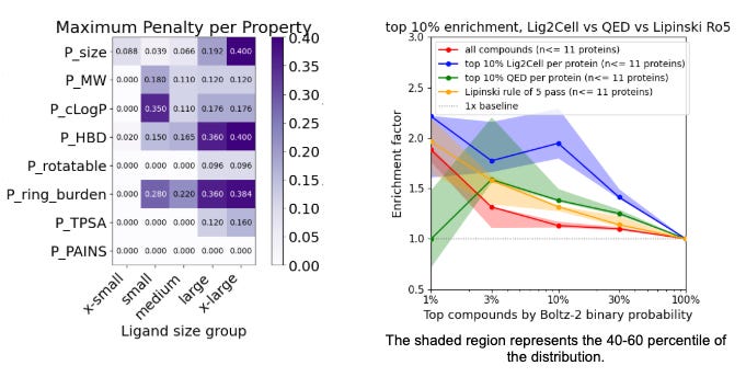
Hopefully I will get to open-source the score 🤞. But first, I need to evaluate it more thoroughly, and run more co-folding for x-small, large, and x-large compounds to reduce the current noise in the curve fitting.
This is the billion dollar question 💰! Who cares if co-folding works for your competitor or colleague, what about YOUR target? Will binding work? And will it translate to cell-based in-vitro assays?
Recursion is again well equipped to answer this question thanks to its massive phenomics dataset.
In this section: I compute the affinity–phenomics agreement separately for each protein, and ask which properties make co-folding more likely to correlate with biology assays. What I observed was quite surprising: protein class, size, domains, and embeddings did not work well. Instead, the most important properties are the gene ontology annotations, which tell us where a protein is, and what is it does.
I use the same data as the previous section, so 500k ligands over 7k proteins at ~1% sparsity. Across all targets, the median AUROC is only 53.9%, showing that affinity captures some biological signal, but is very far from replacing phenomics. But some targets have a much stronger signal than others.
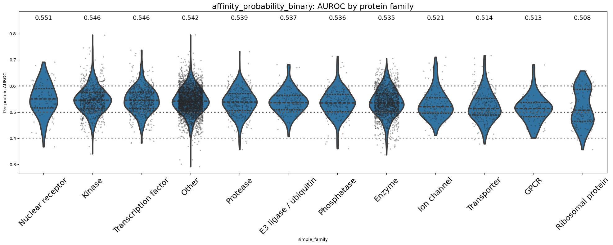
First, let’s do the obvious! Protein family! We heard it many times “co-folding works on Kinases but not GPCRs”. Well, it’s wrong! Sure, on average, kinases are one of the best classes, GPCRs are one of the worst, but we find a very strong overlap between each class. This means that choosing a program based on the protein class is not a good approach. Co-folding can work and fail on any.
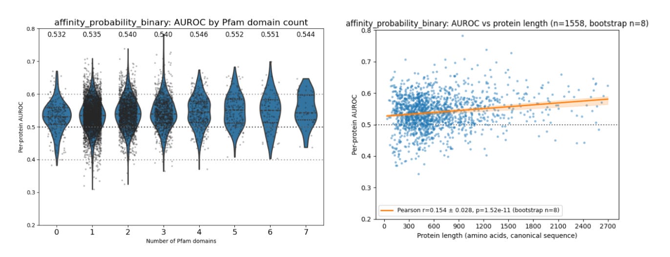
What about protein sizes or number of domains of the protein? Surely bigger proteins will not work as well because there are more mistakes and misplacements that can happen? Wrong again! Looking at the two figures below, we find no correlation between the protein size or number of domains. 🤔 Weird. But let’s remember that our segmentation is likely to split large proteins into 2-3 segments, then max-pool over their affinities, so large proteins are split into smaller bits.
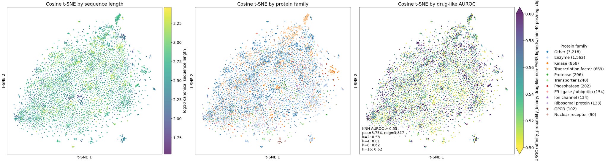
I know! ESM2-3B embeddings will clearly create visible clusters of where it works, and a simple KNN would be able to disambiguate between them? Wrong again! You can look at the TSNE projections in the appendix.
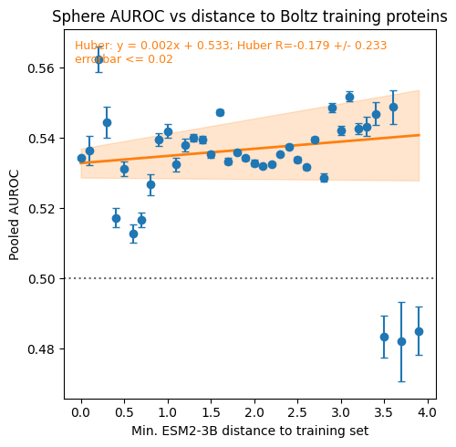
Maybe the distance to the training set? Wrong again, the correlation is mostly flat between the distance to the training set, and the AUROC. See the result in the appendix.
So I kept going. I tried many properties, some coming directly from the sequence and others computed from the AlphaFold-DB structure. And although some properties showed promise, like GRAVY, and SASA, they only helped with certain protein classes that interact with RNA or lipids, like ribosomal proteins and GPCRs. But for kinases and transcription factors? Still nothing… Except for a few classes, we still can’t tell which target will better translate between affinity and phenomics.
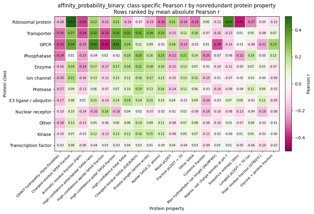
So I asked myself: maybe what the protein looks like doesn’t matter too much, maybe where the protein is located matters more? Perhaps certain compartments in the cell are harder to reach, or less visible from a phenomics perspective, or more critical, or more redundant, or have too many unaccounted natural interactions. In this next step, I took different feature sets: Domain, class, calculated properties (from the plot above) and gene ontology (GO). The GO annotations are separated into “cellular-component” (the where it is) and “molecular-function” (the what it does).
Gene ontology looked much more promising than protein class or structural properties, so I tested whether it could predict which targets translate well. I trained a RandomForest using different feature sets: GO annotations, domains, protein class, calculated properties, and ESM2 embeddings.
The task is to predict whether the affinity–phenomics AUROC is above 0.55, using 10-fold cross-validation stratified by protein class. Essentially, we want to predict on which target the affinity-prints correlated significantly with the Phenomics maps, and we measure the classification success with class-balanced AUROC.
What I found is that the single most important set of inputs, by far, is the gene ontology (GO), especially the cellular component (the where it is)! And using all GO together yields the same performance as using the whole ESM2-3B embeddings, despite being only a 50-dimensional binary vector compared to a very rich float embedding of 2560 elements. On the other hand, protein domains and classes perform only slightly better than random.
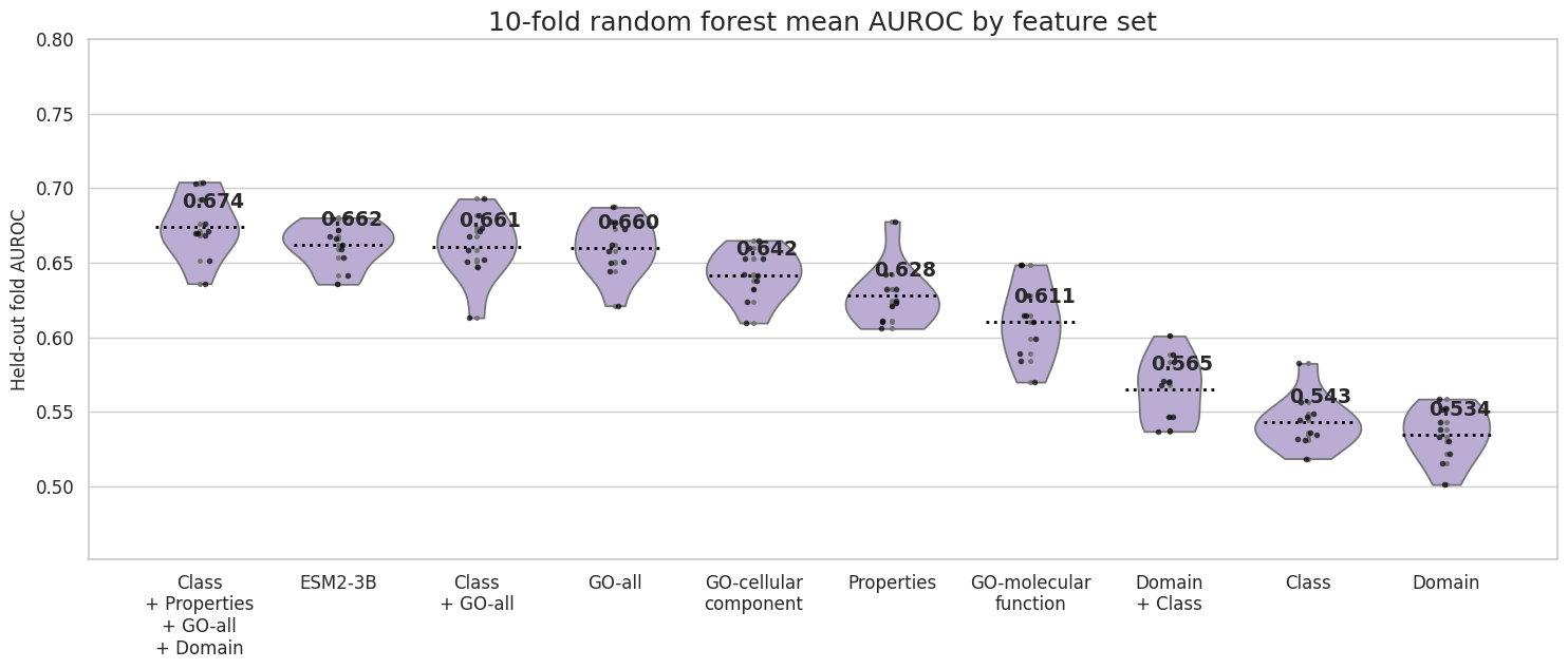
Although far from perfect, I built a decent and simple predictor that explains, with simple rules, where affinity-prints are likely to translate well to phenomics assays. As a sanity check, I tested as input the GO count for each category, and the average AUROC was 0.526, so the model is not simply learning “more annotations = better target”.
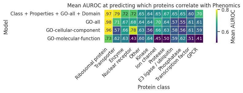
I also find that gene ontology (GO) is more than sufficient for most classes, while other properties matter mostly for Transporters and GPCR (where lipid presence matters), Enzymes and Phosphatase where pLDDT can predict disordered regions, and E3 ligase.
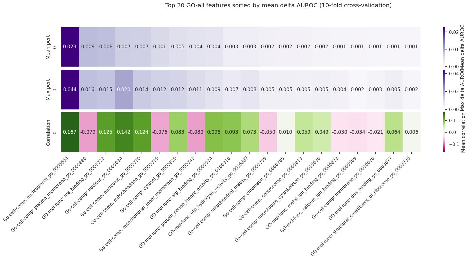
I then decided to measure the perturbation importance, which shuffles a single input at a time and measures the drop in AUROC at inference time. I find that the GO properties that mostly drive good affinity / phenomics translation are: nucleoplasm, nucleus, and nucleolus; while they translate worse for mitochondrion and mitochondrion membrane.
We also see that GO molecular functions of ATP binding and RNA binding (ranking 9th and 10th) are very important decision makers, way ahead of the Ribosomal protein and Kinase classes (ranking 26th and 29th) that are typical ATP and RNA binders. This is strong evidence that the target’s function matters more than its class.
More about these results in the appendix.
So why does the gene ontology (GO) annotation explain so well which protein targets are most correlated with binary affinity? Unfortunately, I don’t have a good answer for that, all I can do is give my best guesses below:
Accessibility: Where a target is located impacts how difficult it is for a ligand to reach its target at enough concentration. For example, the mitochondrion has a dual membrane, which requires different ligand properties to cross.
Criticality: Where a target is located impacts its likelihood of being critical for the cell function. For example, targeting nuclear proteins is likely more critical for a cell’s survival than a mitochondrial protein.
Prior knowledge: A target’s function impacts the kind of interactions that drive its function, and some might be easier to target based on prior knowledge, like ATP binding sites.
Inhibition /= loss of function: Our data compares ligands inhibition to GeneKO, which holds well for catalytic roles, but breaks down for receptors or signaling proteins.
Readout visibility: Some cell compartments are likely easier to image and capture by deep learning models… Which is one of the reasons that I should have been using the newer Phenom-2 map 😥.
I would be happy to hear your thoughts on this.
Co-folding models provided a step-function change in our understanding of chemical interactions and binding affinity. However, this is far from being solved as there are plenty of issues remaining in terms of generalization. And they can’t be solved blindly by scaling the models, they span from noisy and sparse public data!
First, Boltz-2 struggles more on proteins with large lipophilic surfaces. X-ray structures often remove the lipid environment and capture only one rigid state, giving the model an incomplete picture. Fixing this will likely require better engineering and more simulations.
Second, crystal structures are sparse. The recent Runs N’ Poses benchmark showed that novel ligands are often placed incorrectly in the pocket. Since new x-ray structures are expensive, I expect more hybrid co-folding + molecular dynamics methods to correct poses and generate better training data. This is a strong fit for Recursion, with our combination of compute, MD, and ML expertise.
Third, affinity data is also sparse, especially full IC50 curves, and most high-quality datasets are private. Docking can expand the space but is noisy; MD is better but not scalable. Recursion’s phenomics maps could help prioritize which chemical space is actually worth exploring.
There are still a lot of challenges along the way in terms of co-folding, but also in terms of bridging affinity models with biology. I enjoyed playing with the affinity-prints, but there are still a plethora of things to try. Fortunately, Recursion is best positioned to tackle these hard questions, with the right balance of ML, MD, compute, and most importantly, biological data. Indeed, as co-folding models keep getting better, the real advantage is understanding when and why they fail to translate to real biology.
Big thanks to Ali Denton, Cas Wognum, and Emmanuel Noutahi for their help with biological data and insights, Stephan Thaler for running the protein-protein interactions, to Austin Tripp and Julien Roy for recommending more ideas to try and biases to analyse.
Massive thanks to Claude’s Fable-5! By refusing to help me write the blogpost, you really helped keep the world safe! ♥️
Hey reader! If you’re still here, there’s some extra plots for you. I didn’t want to bore you by showcasing everything all at once.
As we can see, the ECFP map doesn’t look nearly as good, because it only captures a few key compounds that are highly similar, not the full distribution. Furthermore, the ECFP maps can’t be adapted on a per-cell-line basis, making it a major limitation.
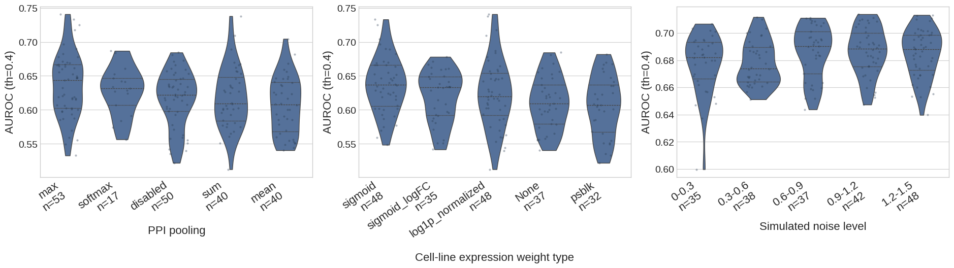
Below I show a small ablation study. I ran multiple random WandB sweeps trying 2,000 different parameters of design decisions and hyper-parameters, with only uniform distributions. I then isolate the top 200 runs of each sweep and look at the distribution of key components. Although there is a large overlap between the different choices, we clearly see that the top models all use PPI pooling, cell line expression, and simulated noise levels.
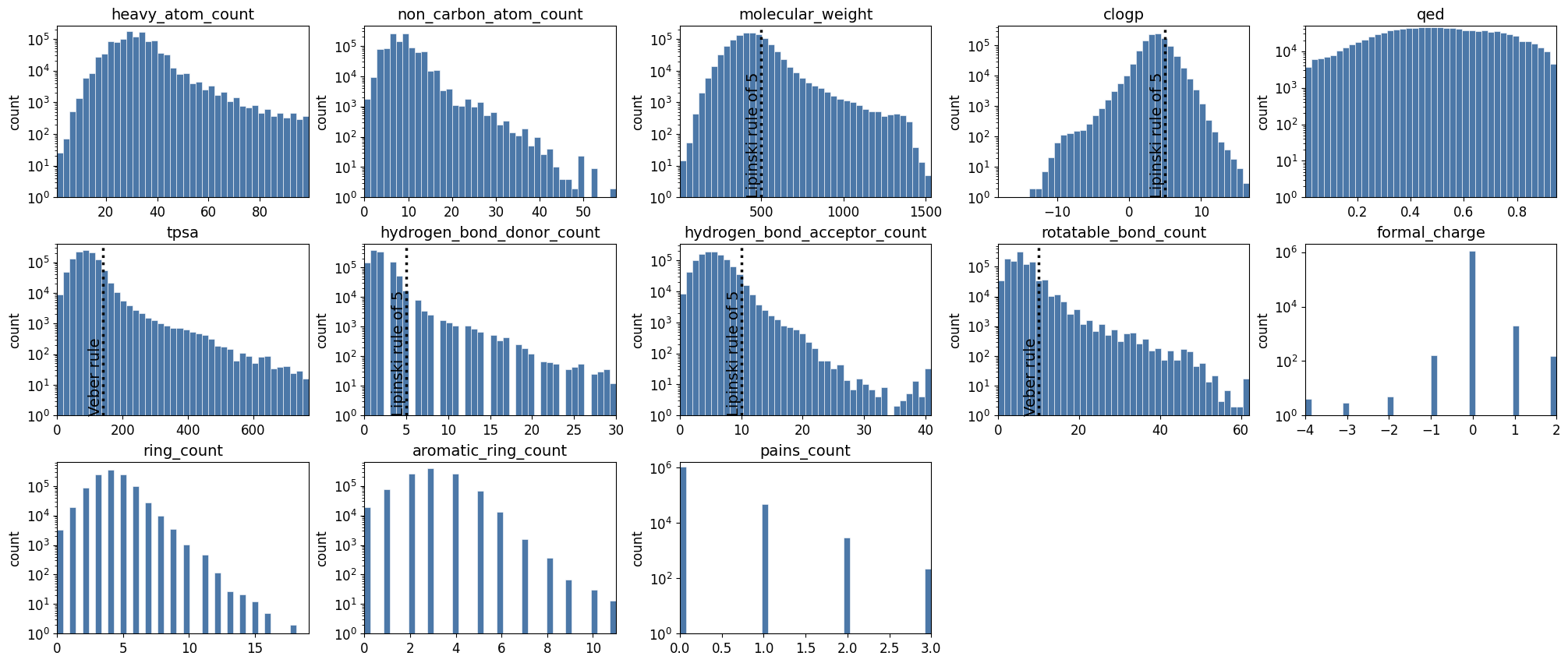
After analysing the effect of ligand properties on the performance degradation, one of the main criticisms I was getting was that it could be an artefact of the training data from Boltz-2, rather than the difficulty translating to phenomics. So let’s look at the histograms! For simplicity, I removed every compound with >100 heavy atoms prior to plotting the distributions.
First, we notice that the training data expands way beyond the Lipinski rules of 5, while our plots showed a direct intersection there. Second, we note that the number of compounds drops a lot at <20 heavy atoms or <2 cLogP, while our data shows an increase in AUROC a little beyond these points, before the data becomes too scarce. Then, we see an almost uniform QED distribution, with a peak at 0.5, while our data shows a small but upward trend. For ring counts and aromatic ring counts, the data peaks close to the limits that we found, contradicting the hypothesis of a training data issue.
In summary, I found no evidence that the curves were simply representing the generalization and training data regime of Boltz-2.
Despite ESM2 creating beautiful clusters for protein classes (see sanity check on the left), its KNN predictions for whether affinity will correlate with Phenomics maps are only a little better than random. And on many protein classes, like Kinases and Transcription factors, the KNN is giving random results.
In the figure below, the AUROC in blue represents the targets for which binary affinity predictions correlate with phenomics, and in yellow, those where the correlation is weak.
One of the most typical approaches for measuring the distance between the inference set and the training set.
We see no evidence that the target distance to the training set affects how the Boltz-2 binary affinity predictions translate to phenomics. This is surprising since there are studies that found that the co-folding performance depends on the distance. However, note that this result is limited to human proteins from the phenomics map.
In this section we show the protein feature importance of the RandomForest models in determining which proteins will translate well to cell assays.
Interestingly, pLDDT is very important and negatively correlated, showing that disordered and flexible proteins are more amenable targets. However, one must remember that our methodology segments out the disordered regions before running co-folding, so the disorder here might be a proxy for protein importance within the cell. Also, the negative correlation does not imply that the RandomForest uses it negatively.
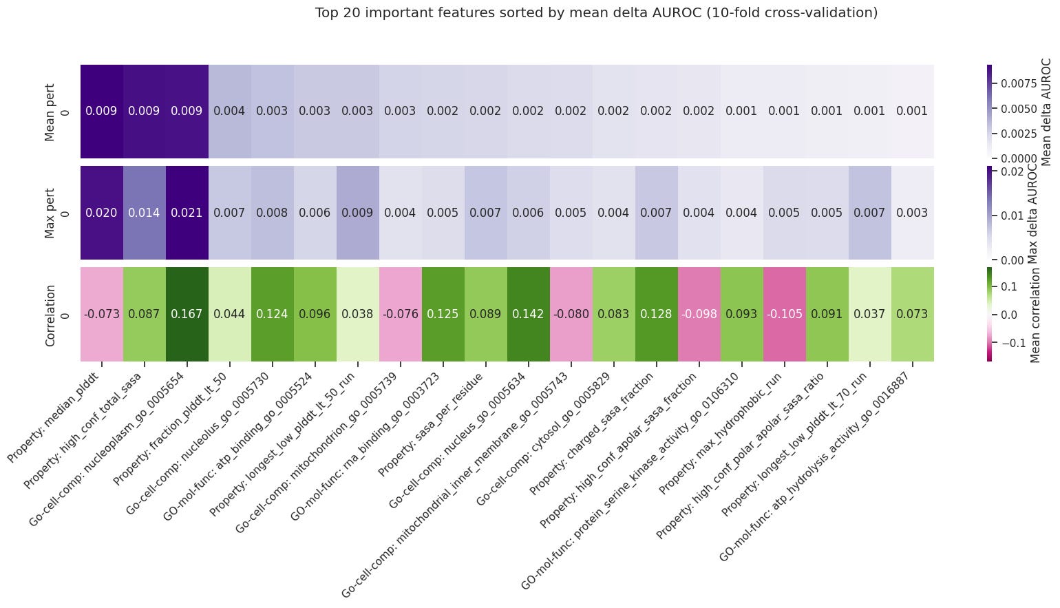
When looking only at the GO-only model, in the figure below, we see a slight change in the ranking. For example, “Plasma membrane” now ranks #4 but it was not in the top-20 properties before. This is because it is redundant with other properties, such as SASA, that better predict binary affinity to phenomics transferability than simply its location. So being on the membrane is an important indicator, but how much membrane lipids cover the surface is a better indicator.
For brevity, I’ll showcase 5 examples
Comments
Nothing yet. Say the first thing.
Sign in to join the conversation.