Schrödinger’s Macro Lens #1

To make it easier, I also launched a site: schroedingers.ai, updating Saturday allocations and (eventually) crypto and stock picks.

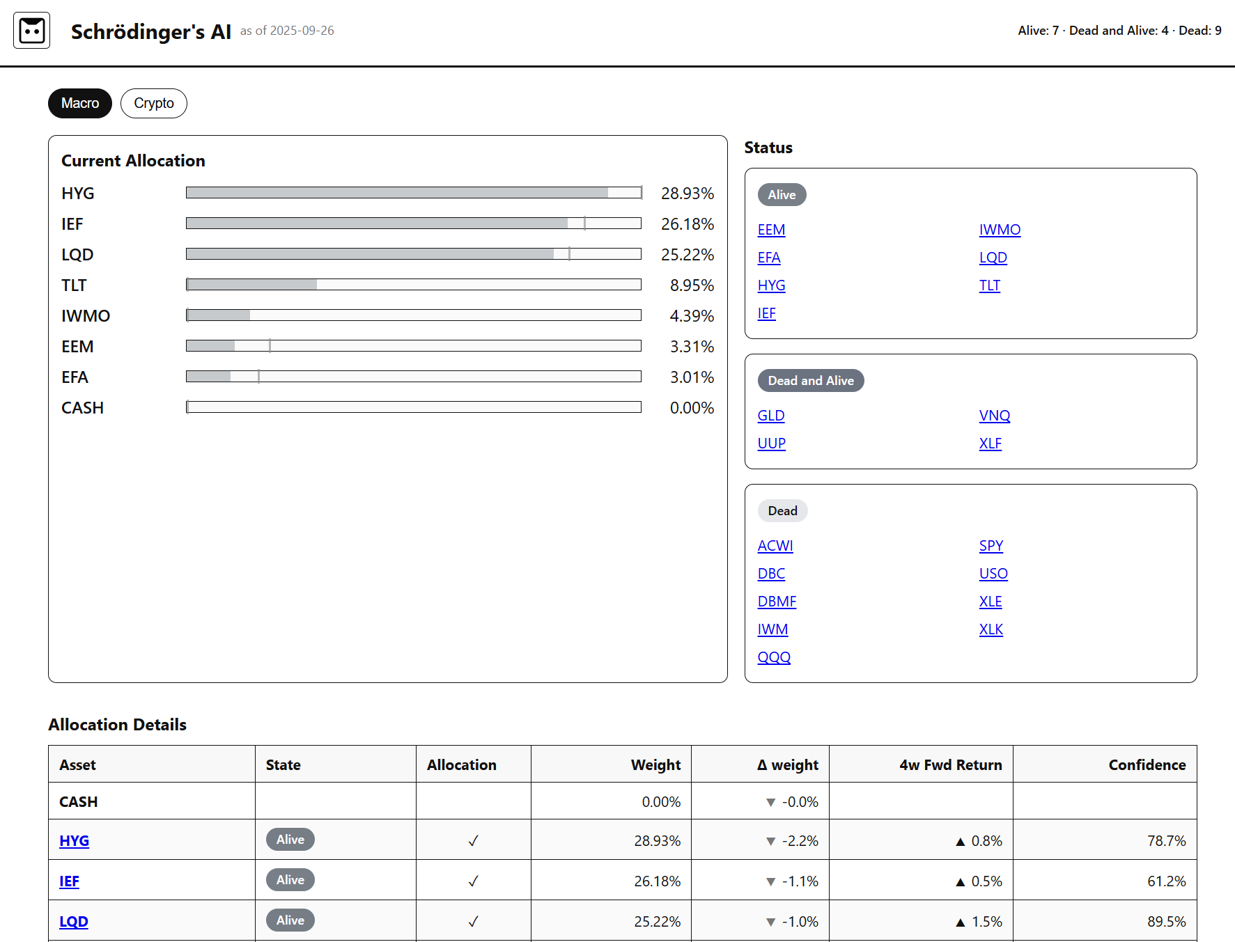
• Alive this week: HYG, IEF, LQD, TLT, IWMO, EEM, EFA.

• Deallocated: DBC (commodities).

• New addition: TLT (long US Treasuries).

• Portfolio tilt: ~80% bonds, strong income/defensive stance, with a reach into high yield credit (HYG). Small equity allocations via EM (EEM), DM ex-US (EFA), and a momentum factor tilt (IWMO).

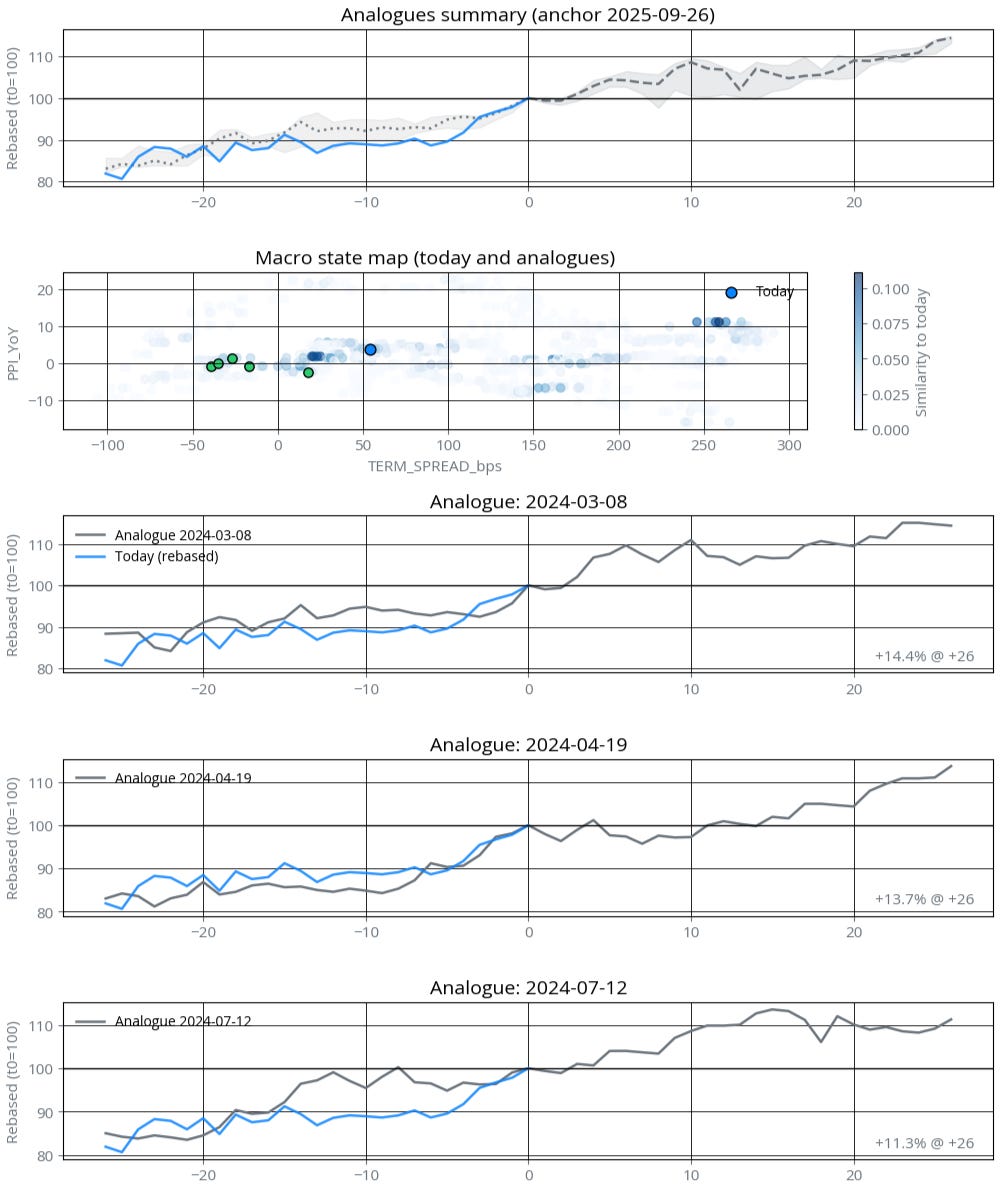
• Gold sidelined: short-term analogues were bullish, but most came from inverted-curve regimes in 2024. With today’s 10y–2y spread back in positive territory, the macro backdrop doesn’t match.

• Silver would have fit better in this macro setup (more cyclical, reflationary profile), but it’s excluded from the ETF version for tax reasons, so the allocation went to bonds instead.

• Crypto cautious: Bitcoin and Ethereum remain Dead for now; analogues point to sideways near-term, with potential only emerging after ~10 weeks.

• Factor importance: Decisions are ~60% driven by price dynamics (trend, volatility, drawdowns) and ~40% by macro factors. Most important single macro factor this week: the 10y–2y yield spread.

Here’s how Schrödinger has placed its bets:

Bonds (~89%)

• HYG (29%) – high yield, risk-seeking within credit

• LQD (25%) – safer corporate credit

• IEF (26%) – core intermediate Treasuries

• TLT (9%) – new addition: long duration Treasuries

Equities (~11%)

• EFA, EEM – international and emerging market exposure

• IWMO – momentum equity factor

Commodities (~0%)

• DBC removed this week

• The cat is playing it safe overall, but still reaching for yield via HYG.

• Minimal equity: the model remains cautious on U.S. equities, only small tilts in EM, DM ex-US, and momentum.

• Gold excluded: despite strong short-term signals, the longer-term analogue context didn’t line up.

• Silver might have been the better fit under today’s positively sloped curve, but since it’s not part of the ETF portfolio (tax inefficiency), the model had to pass entirely.

• Bond-heavy tilt: the Alive roster is ~80% fixed income, consistent with a regime where a normal yield curve favors duration and credit.

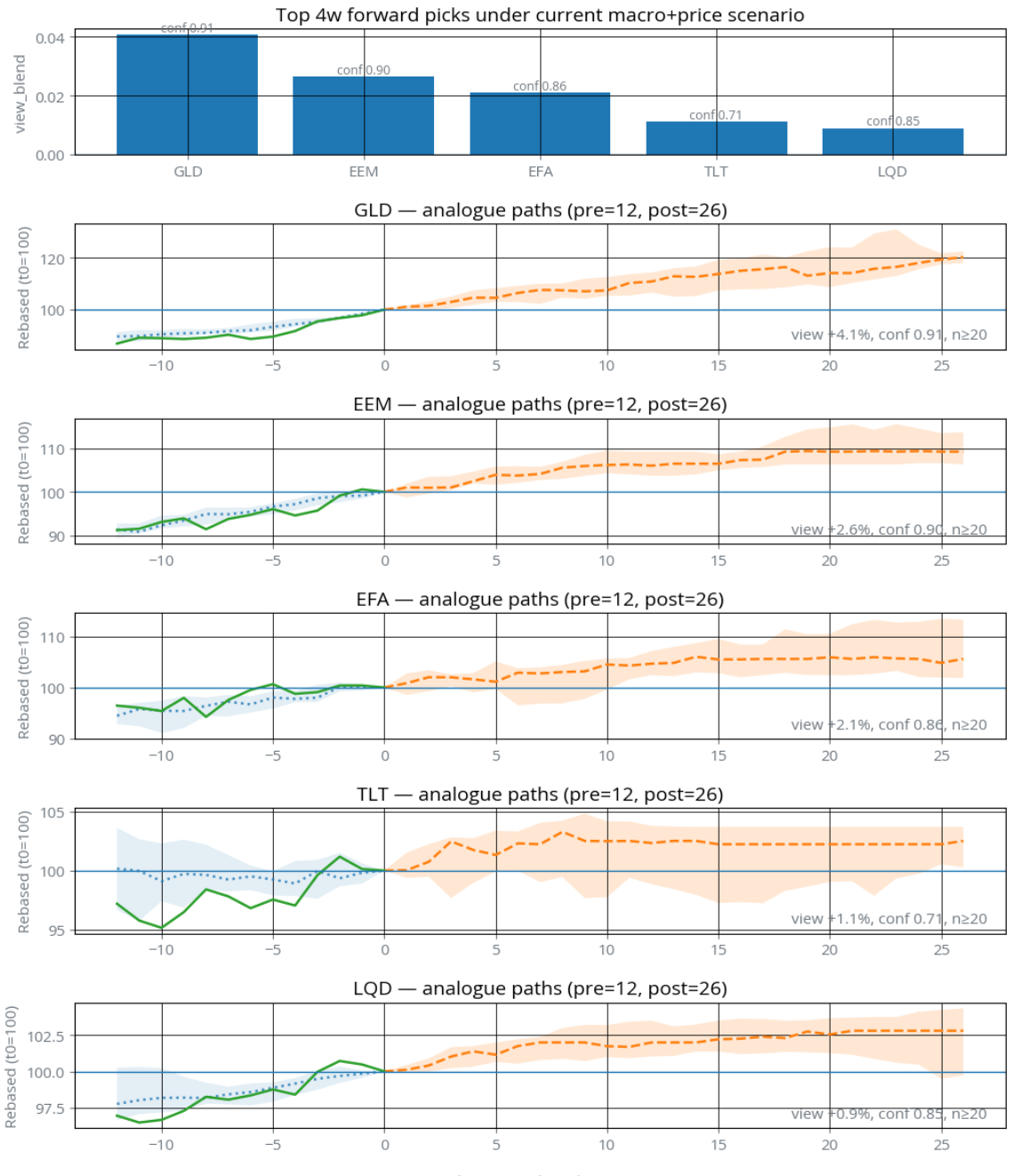
The answer lies in the longer horizons. Beyond 4 weeks, the analogue paths for Gold became much less consistent, with bullish and bearish outcomes mixed together. Most of the bullish matches came from 2024, when the yield curve was inverted. Back then, a flat or inverted curve signaled recession fears, a macro backdrop where Gold often thrives as a hedge.

Today, the story is different: the 10y–2y spread is back in positive territory. A positively sloped curve historically aligns more with normalization and easing growth risks, regimes where bonds often do better than Gold. That shift might explain why the model lost conviction beyond the near term: the macro backdrop today simply doesn’t line up with the bullish analogue histories.

Put differently: price said “buy Gold,” but the macro lens disagreed.

Interestingly, the model’s analogue matches suggest that Silver may be a better fit in today’s environment. Unlike Gold, Silver tends to behave more cyclically, with stronger ties to industrial demand and reflationary phases. In past regimes with a positively sloped yield curve, Silver showed more consistent follow-through.

In other words, Schrödinger’s lens sees “growth proxy” where Gold was more of a “crisis hedge.”

For now, though, this is a missed opportunity. Silver isn’t part of the ETF portfolio I’m running here, mainly because of tax inefficiencies. So in practice, the cat had to choose between Gold or nothing. And this week, the answer was: nothing.

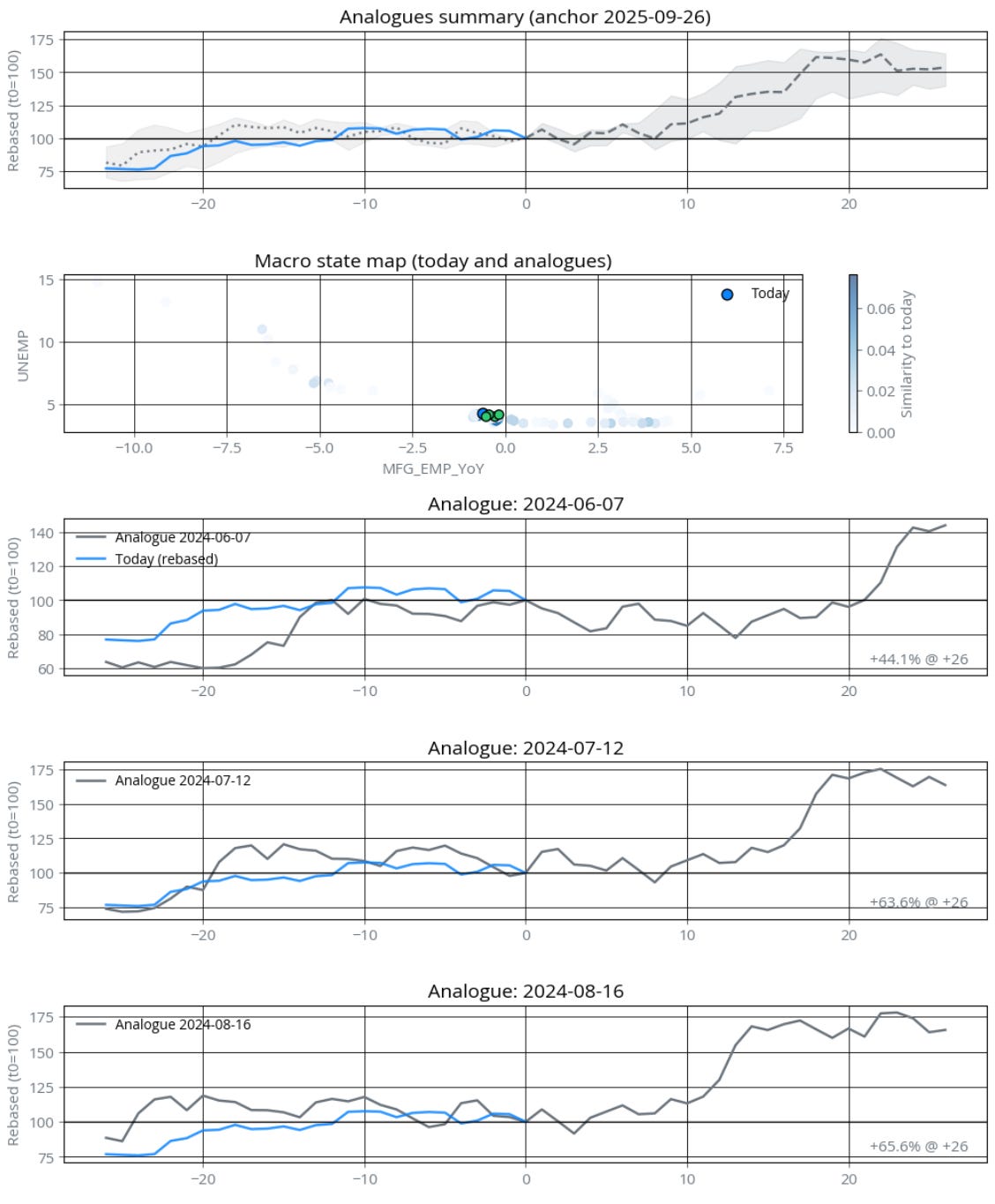
Bitcoin’s case is even trickier. The analogues are dominated by recent episodes from 2024, despite the model having more than 10 years of BTC history to chew on. Most of these episodes show Bitcoin drifting sideways in the first few weeks before picking up only after ~10 weeks. That pattern could reflect its higher sensitivity to liquidity cycles, when yield curves steepen and policy looks less restrictive, BTC sometimes lags before catching a bid. For now, Schrödinger classifies it as Dead, but with a clear note in the margin: “potential Alive later.”

Schrödinger’s AI works by comparing today’s market “fingerprint”, a mix of price dynamics and macro context, with thousands of past weeks. It then asks: when markets looked like this before, what tended to happen next? From those analogues, it builds short-term (4, 8, 12 week) forward scenarios. If the evidence is strong and consistent, the asset is classified as Alive (eligible for allocation); if not, it’s Dead. Position sizes are then scaled by signal strength, volatility targeting, and diversification rules.

1. State construction - the market’s fingerprint
Each Friday, every ETF is described by a feature vector capturing price (momentum, volatility, drawdowns) and macro context (yield curves, spreads, inflation, employment, industrial production).

2. Self-similarity - who looks like me?
The model compares today’s fingerprint with past states using distance metrics (Euclidean / Mahalanobis). The closest analogues are retained.

3. Conditional forecasts - what happened next?
For each analogue, the model looks forward 4, 8, and 12 weeks to collect possible outcomes and return distributions.

4. Horizon blending - weighting the near term
Forecasts are combined, with heavier emphasis on nearer horizons (4 > 8 > 12). This keeps the model responsive but grounded in context.

5. Alive/Dead filter - the cat decides
To qualify as Alive, an asset must have:

• Enough analogues

• Consistent forward returns

• Sufficient confidence and magnitude

Weak evidence = Dead. Conflicting = Alive & Dead (Schrödinger’s paradox in action).

6. Relative strength sizing - conviction matters
Alive assets are ranked by signal strength. A logit-power transform emphasizes strong views without going all-in.

7. Portfolio controls - keep the box stable
Volatility targeting (~15% annualized), position caps (max 40%), and diversification checks avoid concentration and smooth performance.

Intuition
Schrödinger is a historian, not a fortune teller. It doesn’t predict in the abstract; it recalls past regimes that looked like today and borrows expectations from them — but only when conviction is high.

With the mechanics in place, the next question is: what markets does the cat actually watch? For accessibility, I built a compact ETF universe that captures the major macro dimensions without overwhelming readers with hundreds of tickers.

With the mechanics in place, the next question is: what markets does the cat actually watch? For accessibility, I built a compact ETF universe that captures the major macro dimensions without overwhelming readers with hundreds of tickers.

• Equities: broad US (SPY), small caps (IWM), tech (QQQ), international developed (EFA), emerging markets (EEM), and a momentum factor tilt (IWMO). Together, these capture growth cycles, regional dynamics, and style effects. I left out other equity factors for now - well, I’m a trend-follower and momentum guy after all.

• Fixed Income: Treasuries across the curve (TLT, IEF), investment grade credit (LQD), and high yield credit (HYG). This sleeve reflects policy, inflation, and credit risk dynamics and as this week shows, it can dominate when defensive signals prevail.

• Sectors & Real Assets: Energy (XLE), Financials (XLF), Real Estate (VNQ), Tech (XLK). These provide cyclical tilts tied to specific macro drivers (oil prices, rates, credit conditions).

• Commodities: broad basket (DBC), plus targeted exposures like Gold (GLD) and Oil (USO). These hedge inflation and capture supply-demand shocks.

• Currency: USD Index (UUP), representing global liquidity and risk aversion.

• Alternatives: DBMF as a managed futures proxy, offering diversification and a benchmark for systematic trend following. Ideally, I would have used TFPN by Jerry Parker for its pure, classic trend approach. But since I want this portfolio to be live-tracked in my brokerage account, I needed something that’s easily tradeable in both the US and EU.

This universe is deliberately broad but not sprawling. Around 20 ETFs that together span growth, inflation, policy, and risk-on/risk-off. It’s designed so anyone with a brokerage account can follow along.

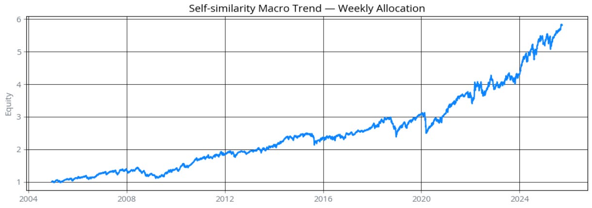
Before diving into crypto, a quick word on how the analogue allocation has behaved in backtests. With slippage and transaction fees included, the model produced Sharpe ratios in the 0.9–1.2 range, depending on aggressiveness and rebalancing frequency.

For live tracking, I settled on a less frequent rebalancing schedule and a target volatility of ~15%. The goal is to make the portfolio relatively insensitive to execution delays, most bets are designed to play out over weeks, not days.

The results below reflect only the ETF universe, crypto is not yet part of the allocation.

• CAGR: ~14–15% after costs

• Max drawdown: ~24%

• S&P correlation: ~60%

That higher correlation to equities arises naturally from the ETF design. Unlike the broader futures-based Macro Trend backtest, which could lean more heavily into commodities or even short equity indices, the ETF version is long-only and structurally carries more equity exposure. With fewer diversifying sleeves (like commodities and FX), it will tend to move more closely with traditional stock/bond allocations.

For now, I’ve only seeded Schrödinger’s crypto notebook with a handful of liquid assets: BTC, ETH, and a small selection of majors like DOGE, XRP, SOL, SUI, and HYPE. That means Schrödinger’s choices are limited at this stage, it can’t yet roam the full crypto jungle.

Even so, the analogues are fascinating. Despite a 10+ year history for BTC, the model’s closest matches right now are surprisingly recent (2024), which explains why it’s cautious near-term but hints at potential 10 weeks out. As I expand the crypto universe in coming weeks, the model’s calls will naturally get richer and more nuanced.

• Weekly ETF allocations posted every Saturday on schroedingers.ai

• Monday writeups with charts, macro maps, and signal stories

• Extension to single stocks universe and refined crypto logic

• The cat continues to explore, maybe one day it’ll meow in human tongue

Your Turn: Watch for the next post: we’ll drop the full allocation charts and interpret the drivers in each “Alive” call.