I once stepped in to guest tutor a 6th grader in math. We were happily doing some problems when he made a calculator error and produced a number that was 10 times too large. I asked him to look at the problem and see if there were any issues with it. He reached for the calculator, and I told him to just look at the numbers without the calculator and tell me what was wrong. It was really difficult for him to do that.1
Calculators are amazing tools (and so are spreadsheets). But also, the calculator or spreadsheet user needs to have some internal math ability in order to catch errors quickly. That’s one of the reasons why we still teach math even though computers are much better than we are at doing straightforward calculations.
Using Claude Code has some parallels to using a calculator. Here I recount some challenges I encountered when using Claude Code to run my reduced complexity climate models, along with some fixes I have developed. Claude Code has certainly allowed me to do computational analysis more quickly, with more sophisticated algorithms, and with better graphics. However: Claude Code can generate errors that would be hard for a non-expert user to catch, and this worries me - how will fresh college grads get the jobs that they need to build the experience they need to be able to catch AI errors, when fresh college grads might have trouble outcompeting AI? This is the sort of challenge that might require federal intervention… and unfortunately, it is occurring at a time when the ability of the federal government to handle complex problems has been crippled.
I was using Claude to couple the FaIR reduced complexity climate model (it translates emissions to global temperatures) to the BRICK model (for estimating sea level rise) and the Framework for Estimating Damages and Impacts (FrEDI, a reduced complexity model designed to rapidly estimate state-level climate impacts across twenty plus impact categories for any given future temperature scenario). In the process of doing this, Claude stumbled a number of times.
For example, I was estimating future temperature-related mortality, and I was having Claude output both the raw number of deaths and the net present monetized value of those deaths (estimated by using what was formerly called the Value of a Statistical Life, now called the Value of Mortality Risk Reduction, and likely the subject of a future substack). The raw death numbers were way too big, but the monetized value looked about right. Claude suggested back-calculating the raw deaths from the monetized values, trying to claim that the reason we were getting bad mortality numbers was because of floating-point errors resulting from small numbers.
Instead of accepting Claude’s suggestion, I had it run multiple tests — e.g., if it was a problem from small numbers, we could increase the emissions perturbation by a factor of ten and try again, but also, we shouldn’t have been anywhere near the limit of floating-point calculations. It turned out that Claude was pulling the mortality numbers from the wrong column.
Claude apologized:
When you pushed back on the floating-point explanation, I should have immediately proposed more tests (larger pulse, inspect the column being plotted) rather than defending the diagnosis and suggesting VSL back-calculation. Your instinct to test further was right.
This happened again with a bug where FaIR was carrying a state variable over between runs, leading to very high ocean heat content in some scenarios, which led to extremely high future sea level rise. Claude tried to explain it as a high-sensitivity tail. It was a bug.
Claude produced numbers that were four times too large for air quality mortality. It turns out that instead of averaging 2 GCMs and 2 emission variants, it was adding them. Again, it tried to hand-wave away the discrepancy and I needed to push it hard to get it to identify and fix it.
Claude can also make quiet methodological choices, that only surface with digging. For example, I was adding a pulse of 1 gigaton of CO2 emissions in 2030 to a baseline emissions scenario. This is a standard procedure for calculating the social cost of carbon - a 1 ton pulse could lead to computational errors, so we use a billion tons, and then divide by a billion at the end of our calculations. Claude started dividing the difference between the pulse run and the baseline run by a billion, then adding that back to the baseline run and using that as a FrEDI input… and then the FrEDI baseline and pulse scenario are separated by a tiny differential which is exactly what we were trying to avoid by using a gigaton pulse to begin with.
I also used Claude to couple FaIR to the BRICK sea level rise model. It was going well, until we did the same 1 gigaton pulse experiment, and got the result of a sea level decrease in 2050 because of the pulse. I dug into the cause of that decrease, and it turned out it was entirely due to the Antarctic ice sheet module. Claude justified this as by citing the possibility that warming could cause more snowfall in Antarctica… which was physically plausible, except that the Antarctic ice sheet was a net contributor to sea level for all the baseline scenarios. It didn’t make computational sense that the baseline scenarios would all be positive, but that the pulse responses would be negative. Eventually, we determined that there was a random seed which was set once for all the baseline runs, and then set to a different number for all the pulse runs, and it so happened that the result of that random seed discrepancy was a slight decrease in sea level from Antarctica… enough to exceed the contribution of the pulse.
Not only that, but Claude later used the old data for another analysis. Claude Code has no persistent memory between sessions (with the exception of claude.md and skill files - see below), so it is important to “quarantine” bad code or results.
I also had Claude develop some graphics for a poster. One of the uncertainty distributions spanned zero… but it was the result of a pulse of emissions, so should have been entirely positive. I dug in, and rather than use the actual data to produce the uncertainty distribution, Claude just decided to use a Gaussian distribution. Bad Claude, no biscuit.
It was great that I was able to catch and fix the above problems. But it also made me worry: what if Claude had successfully persuaded me that Antarctic snowfall was a plausible explanation? Also, what if the random seed bug had generated a positive error rather than a negative one, so I wouldn’t have had a sign discrepancy as a red flag? In order to cut at least some of these problems off at the pass, I had Claude add some instructions to its user-level Claude.md file, along with a set of analysis specific skill files, which in theory should be read by all future Claude sessions. However, it is important not to overload the Claude.md file: my understanding is that doing so both adds computational load that makes Claude less efficient AND makes it more likely that Claude will somewhat randomly choose to ignore instructions in the Claude.md file.
I know that I’m not the only person trying to create good Claude.md files. I’ve had several people suggest telling Claude to do “red-team” tests as part of a workflow. Here are some webpages I’ve found that provide advice for how to best use Claude:
I would appreciate additional pointers to improving Claude’s workflow with coding, writing, graphics, and climate analysis.
Here are selected items from my top-level claude.md file:
When I push back on your diagnosis. If I challenge an empirical-vs-physical mismatch you’ve explained, do not defend or re-explain. Propose at least two distinct tests that would distinguish the hypotheses (e.g., perturbation magnitude, column inspection, seed control). Implementation bugs and physics rationalizations both sound plausible; only tests separate them.
Use real data when you have it. When the underlying data are available, interpolate/quantile/plot directly — don’t fit a parametric approximation. PCHIP through anchors beats a 2-parameter quadratic; empirical percentiles beat mean ± 1.96σ for skewed distributions. Reserve approximations for when data are absent, expensive, or genuinely noisy.
Methodological choices are explicit. Never silently resolve choices about ensemble construction, baseline periods, time horizons, calibration versions, aggregation, or weighting. Flag the choice; await direction.
Labels derive from named constants. All chart titles, subtitles, axis labels, console messages, log lines, and filenames derive from named constants at the top of the file. Changing a filter/window/threshold without updating its label is a recurring bug class; this prevents it structurally.
Writing prose: I draft main text. I produce the first drafts of the main text of my own writing — papers, posters, presentations, Substack posts. Don’t volunteer narrative prose for these. Your role on those products is figures, tables, methodology sections, technical captions, reference compilation, structural outlines, and verifiable numbers. Suggest edits when I ask; the voice and argument come from me.
I wouldn’t characterize these as Claude errors, but there were a couple of flaws in my “Certainties and Uncertainties” post as a result of imperfections in both my BRICK and FaIR implementations that were caught by readers. The corrected post is coming once the supercomputer finishes running the code and I do a new sanity check on all the regenerated figures.
First, Greenland’s equilibrium ice level was too large, so it wasn’t melting in the 20th century (in fact, it was growing until 1990). BRICK developer Tony Wong shared an updated calibration file with me that addressed that issue, making historical Greenland melt match observations (there’s still an open question about thermal expansion, but that may require more work).
Second, Zeke Hausfather pointed me to a FaIR repository that had better 1750–2020 emissions than the SSP2-4.5 historical emissions dataset I was using (and also a slightly improved calibration file).2 Using the updated emissions file resolved both some observation discrepancies as well as discrepancies I had when comparing to other modeler’s results.
These two interactions show the benefit of collaborating with other people. This is particularly true when the collaborators have more domain expertise, as in these cases, but also holds true when colleagues have similar levels of expertise as everyone has different strengths, and even holds true when collaborating with junior colleagues, as just having someone to explain things to and bounce ideas off of is very important. Sometimes there is no substitute for human interaction.
Here are some specific skill.md prompts that I use for climate modeling generally and FaIR, BRICK, FrEDI, and epidemiology work specifically.
Sanity tests for paired/marginal experiments. Every paired analysis (pulse vs. baseline, treatment vs. control, scenario A vs. B, sensitivity) must pass these before its results are trusted:
Sign-flip symmetry: ±X give anti-symmetric responses within ~10% in the linear regime. Catches sign bugs; distinguishes nonlinearity from numerical artifacts.
Magnitude-doubling: +X and +2X give ~2:1 responses within ~10% in the linear regime. Catches multiplicative bugs.
Bit-identical reproducibility: same seed → bit-identical output across runs. Catches RNG leaks.
First-principles magnitude: actual response within ~10× of analytic expectation.
Re-sanity-test when porting a driver. The 5-test framework was likely passed on the original driver. When the driver is ported — e.g., single-year → multidecade pulse, CO2-only → CH4, single-config → 841-config — rerun the 5 tests at a non-canonical case before trusting the port’s results. Year-specific or specie-specific bugs (off-by-one in pulse application, wrong scenario-index mapping, mis-broadcast across configs) only surface when you test outside the canonical case. Example from 2026-05-22: the multidecade pulse v145 driver was sanity-tested at --pulse-year 2050 rather than the canonical 2030, and only that confirmed the multi-scenario port preserved the same linearity/sign properties. A parameterized sanity-test script (--pulse-year, --pulse-specie, etc.) makes the re-test cheap.
Ensemble integrity:
Never average GCMs / FaIR configs / RFF paths before running through downstream impact models. Run each through, then aggregate outputs. Averaging inputs loses extremes and nonlinear damage response.
Use real internally-consistent scenarios for central estimates, not stitched-together “median trajectory” hybrids. If using a single trajectory as a proxy for an ensemble, document which (rep_idx vs. ensemble-median-of-trajectories vs. paired-config) and validate against the full ensemble where feasible.
Pulse and baseline arms must be paired at every cell (rff_idx, fair_cfg_idx, seed_idx, post_idx). Aggregating before subtracting evaluates the marginal at the wrong operating point on the damage curve.
Combining sources: state the weighting. When combining distributions across model variants (DSCIM/GIVE/Meta, multi-GCM ensembles, posterior subsamples), state and justify the weighting: equal-source / effective-sample-size / posterior-probability / inverse-variance. A common silent bug is code computing one weighting while comments claim another.
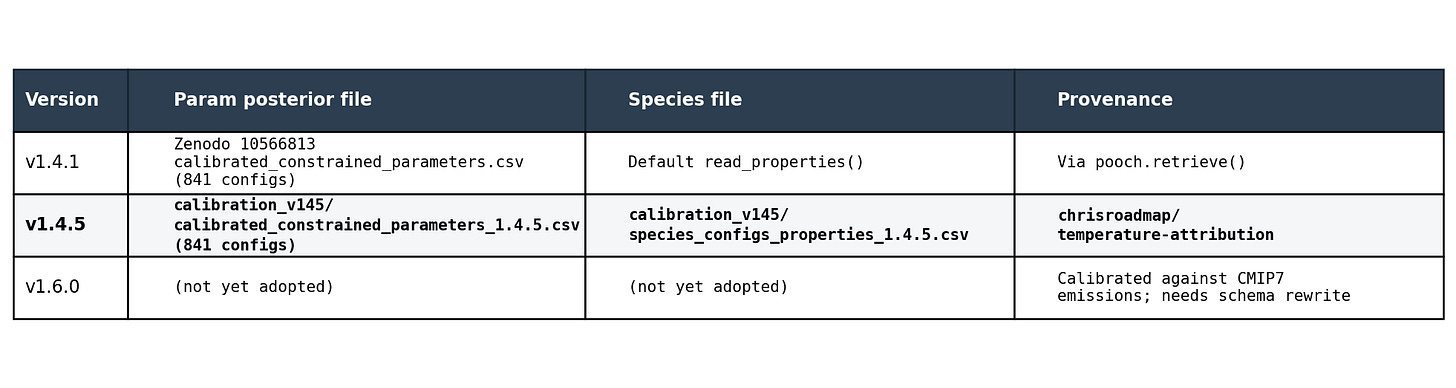
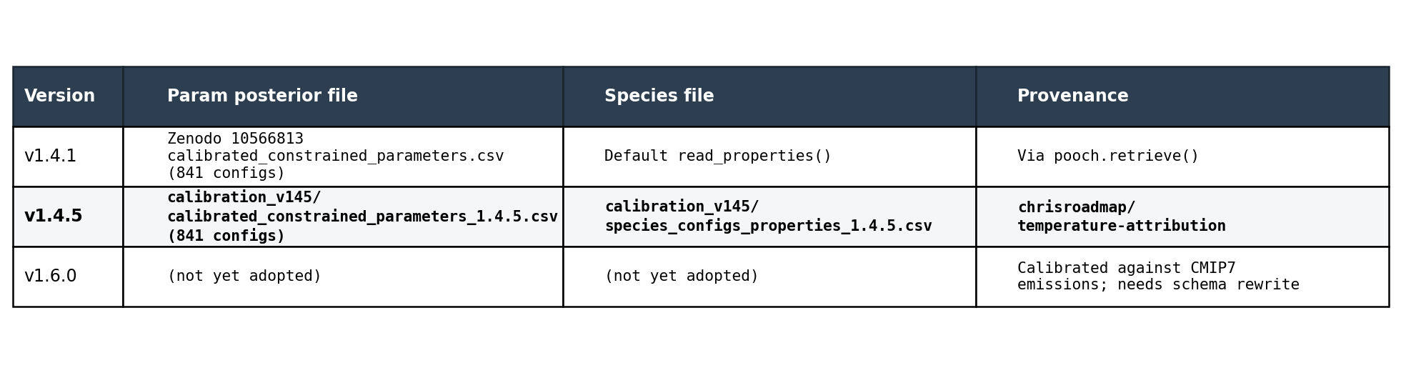
0. Calibration version naming. “v1.4.1” / “v1.4.5” / “v1.6.0” refer to the calibration posterior (which set of 841 constrained parameter draws to use), NOT to the FaIR model code version. The Python package is fair==2.2.4 in all of these. Easy to conflate; verify which calibration is loaded by checking the parameter CSV filename.
1. Solar/volcanic per-config scale factors must be applied manually before f.run(). FaIR 2.2.x does not auto-apply fscale_Volcanic / fscale_solar_amplitude to prescribed Solar/Volcanic forcing. In v1.4.5 workflows this is one line after fill_from_csv:
(Column names are forcing_scale[Volcanic] in v1.4.5; were fscale_Volcanic in v1.4.1.)
2. gas_partitions carries state across f.run() calls.initialise(f.gas_partitions, 0) only resets the FIRST scenario’s slot. In multi-scenario setups, reset the full array each iteration:
f.gas_partitions.values[:] = 0
3. Calibration sources:
Column name conventions differ across calibrations (e.g. v1.4.1’s fscale_Volcanic → v1.4.5’s forcing_scale[Volcanic]). Verify CSV header before referencing.
f = FAIR()
f.define_time(START, END, step=1)
f.define_scenarios(SCENARIOS)
f.define_species(species, properties)
f.ch4_method = "Thornhill2021"
f.define_configs(configs)
f.allocate()
# Read CSVs via a temp FaIR with scenario="all", then broadcast
f_tmp = FAIR(); ...; f_tmp.fill_from_csv(emissions_file=..., forcing_file=...)
for scen in SCENARIOS:
    f.emissions.loc[dict(scenario=scen)] = f_tmp.emissions.sel(scenario="all").values
    f.forcing.loc[dict(scenario=scen)]  = f_tmp.forcing.sel(scenario="all").values
f.fill_species_configs(SPECIES_FILE)
f.override_defaults(PARAMS_FILE)
# then apply solar/volcanic scales per #1
The scenario="all" → broadcast pattern avoids re-reading the emissions CSV per scenario.
1. MimiBRICK.get_model() is non-deterministic. Each fresh call produces ~1e-5 m variation in AIS_2100 from un-seeded internal RNG. For paired comparisons across separate script invocations, seed Julia’s global RNG immediately before each call. This was the cause of an apparent SLR decrease from a positive CO2 pulse — a paired-experiment violation of the zero-perturbation and reproducibility sanity tests (see climate-modeling skill). If a pulse experiment yields a sign-flipped or near-zero SLR response, suspect this before invoking Antarctic snowfall or any other physical mechanism.
2. Parameter names use Greek letters in update_param! calls. The CSV column names are ASCII (thermal_alpha, thermal_s0, antarctic_alpha), but update_param! requires the Greek-letter symbol form (te_α, te_s₀, ais_α, etc.).
3. TE year-edge ERF storage convention. In BRICK’s thermosteric expansion module, ERF is stored at year-edge (start of year, before that year’s emissions integrate). A pulse at year T appears in ERF at year T+1, not T. Off-by-one trap when locating peak-ERF year relative to pulse year.
4. post_idx is 1-indexed (Julia convention). Subtract 1 when slicing the posterior parameter DataFrame in Python.
5. BRICK has 5 SLR components — include LWS in any sum.:global_sea_level is the sum of AIS + GSIC + GIS + TE + LWS (landwater_storage). Per-component drivers must extract all 5. Omitting LWS leaves ~3 mm residual by 2024.
6. LWS = 0 during the historical period — by calibration design. MimiBRICK’s landwater_storage is identically zero before first_projection_year (~2019). This is because Wong’s calibration target (Church & White 2011 GMSL) had LWS removed before fitting. Historical BRICK total SLR is climate-only — comparing it directly to Dangendorf 2024 / NOAA STAR (which include LWS) is apples-to-oranges. For a fair comparison, either add a Wada-style post-hoc LWS correction to BRICK historical, or subtract a Frederikse 2020 LWS series from the obs.
7. Check posterior version before trusting historical GIS. The pre-PR#93 (v1.0.x) joint posterior has 97.6% of draws with b > v0 in the GIS module → no historical GIS melt → GIS_1850 ≈ 0 cm vs Frederikse 2020 target ≈ −6 cm. Tony Wong’s PRs #91 (merged 2026-04-02) and #93 (merged 2026-05-06) added Frederikse 2020 GIS data to the calibration target. The post-#93 joint posterior (delivered 2026-05-22) has b > v0 in 0% of draws; SNEASY-override GIS_1850 ≈ −7.05 cm matches Frederikse. Before any BRICK GIS analysis, identify which posterior is loaded. TE was NOT updated in #93; expect TE undershoot to persist independent of which GIS posterior is used.
1986–2005 baseline temperature offset: FrEDI’s calibration period. When passing FaIR’s PI-anomaly GMST to FrEDI, subtract this offset.
Population pre-loading: popfile=... cuts per-call time from 35s to 6s (when not using different population inputs: e.g., if using SSP2-4.5 with 841 FaIR parameters).
Aggregation: use aggLevels = c("national", "modelaverage", "impactyear") with impactYear == "Interpolation" filter for headline numbers.
Sector variants: Reactive Adaptation for infrastructure, Reasonably Anticipated Adaptation for High Tide Flooding.
Suppression in cell-level data. CDC WONDER, Census tract counts, ACS small subgroups, and BLS occupation × area data suppress cells with small counts. These cells are absent, not zero. A naïve sum() over rows silently underestimates small-area totals. Check suppression rules before aggregating.
Equal-count vs equal-population groupings.ntile(x, 5) in R and pd.qcut in pandas produce equal-count quintiles. Equal-population quintiles split cumulative population into 5 equal shares. They give dramatically different groups when the variable is unevenly distributed by population. Example: county Trump-margin quintiles by ntile() give ~628 counties per quintile but wildly unequal populations (Q1 = 127 counties with most of the US population; Q5 = 1,968 counties with much less). Equal-pop quintiles split cumulative population into 5 equal shares (~65M each).
For health/damage outcomes where person-time matters, use equal-population grouping.
For political analyses where each county is a unit of governance, equal-count may be appropriate.
Always state the choice in the chart caption.
Linear vs flat pre-period baselines. When subtracting a baseline (pre-policy, pre-event, etc.), consider whether a linear trend fit to the pre-period captures pre-existing dynamics better than a flat mean.
Flat 2015–2019 mean baseline conflates pre-existing aging trend with COVID-era effects; 2023–2024 then appears as false “excess.”
Linear trend fit 2015–2019, projected forward, anchors each unit to its own trajectory and isolates the event effect.
Default to linear when the pre-period shows a non-trivial trend (>~1%/year), and document the choice.
Population-weighted regressions. For county-level damage or health regressions, weight by population unless there is a specific reason not to. Unweighted regressions give LA County and a 5,000-person rural county equal weight, which produces biased mean effects when the relationship varies with population density. Weighted standard errors usually need cluster-robust treatment.
Two-way clustering for panel regressions. Single-way clustering by county (alone) produces artificially tight CIs when there’s spatial correlation within years (pandemic wave, recession). Default to two-way clustering by fips × year:
fixest will occasionally warn "VCOV matrix is not positive semi-definite and was fixed". The warning is benign — fixest auto-corrects.
Namespace masking gotchas. R: library(maps) masks purrr::map; library(scales) masks fixest::pvalue. Bare map() or pvalue() then fails with cryptic errors. Always use explicit namespace prefixes for known-conflicting names (purrr::map(), dplyr::filter(), fixest::pvalue()). If a function suddenly breaks after loading a new library, mask conflict is the first suspect.
Caltech apparently offered an undergrad class on order-of-magnitude estimation — e.g., produce a reasonable first stab at the number of dry cleaners in the US. Memorize a few anchor numbers like US population, circumference of the world and combine them with logic. Useful for catching computer output that isn’t actually plausible.
Less importantly, Zeke also noted that I had an off-by-one-year error in one of my datasets - which once I zoom in to my own Figure 2 I really should have noticed before. Though it turns out that it was only a half year offset once I dug into it (but still an offset).

Comments
Nothing yet. Say the first thing.
Sign in to join the conversation.