The hands-on guide to LLM Inference with vLLM

Welcome to the third lesson of the Production OCR course!

If you're new to the course, let me give you a short summary of what we've covered so far …

In Lesson 1, we established the foundations of Kubernetes (what is a pod, what is a node pool, what is KEDA, etc.) with a special focus on how this technology should be used by ML / AI Engineers. After that lesson, you'll understand why traditional software engineering could fall short for AI Systems deployments, as a lot of new issues appear when you are trying to build AI applications.

Then, in Lesson 2, we provided a full overview of the evolution of the OCR field, from 2015 until today, in 2026, ranging from Deep Learning techniques like CRNNs until the hybrid VLM routers we'll be using in this course (and, by the way, one of these architectures you'll be deploying today!).

Now, in this lesson, we want to leave the historical books aside and start getting our hands dirty. So you can expect less theory than the previous article, and more hands-on focus.

To motivate today's topic, let me ask you a question. Suppose I have a PyTorch model that is fully trained on my notebook. If I want to have this model exposed through an endpoint, what would be your approach?

Well … maybe you got it right, but if you ask Miguel from 8 years ago, I'm pretty confident this would have been my answer:

Honestly, there's nothing wrong with this code. I mean, it's correct code, it works great in a demo, or for one single user, running locally on your laptop. But what happens when fifty concurrent requests arrive? Then we have a BIG BIG problem. The GPU starts throwing CUDA OOM errors, latency will quadruple, and, the worst part is that the expensive VRAM you're paying for is holding basically padding, that is, a lot of zeros. You'll be paying a lot of money for A100 to store basically nothing.

Just remember one of our mottos:

AN LLM CALL IN A NOTEBOOK IS NOT A SYSTEM!!

Between the notebook and the system there's a Mount Everest of hardware struggles that most tutorials (typically) skip.

So, our plan for today is to fill that gap. Basically, show you how LLM serving works, the internals of vLLM (the inference engine we're using in this course), and, finally, deploy the real thing … Unlimited OCR on AKS (the most exciting part!!).

💻 The production OCR code is open-source. Support our work by dropping a friendly ⭐ on the repo!

To understand why vLLM, SGLang and TensorRT-LLM even exist, you have to remember how batching worked before generative models came along and ruined everything (I’m being dramatic, but only a little).

Classic deep learning had it easy. Say you're classifying images with a CNN, a ResNet or whatever. The network knows the exact shape of its input ahead of time, so serving is almost boring: collect requests into a batch of 8 or 16 or 32, run one forward pass, done.

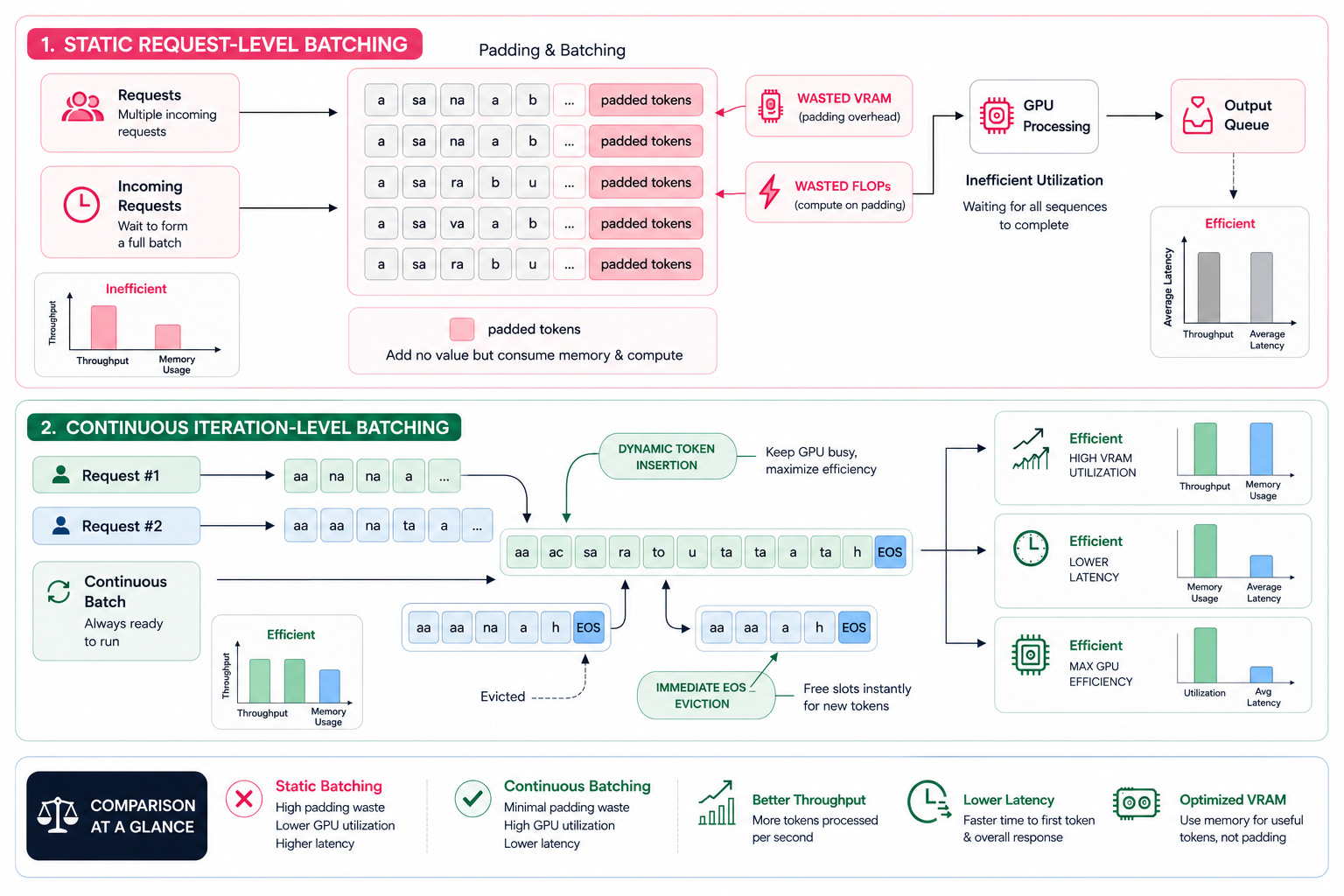
BUT, if you apply the same recipe to a text-generating model … well, the model will break in three different ways simultaneously.

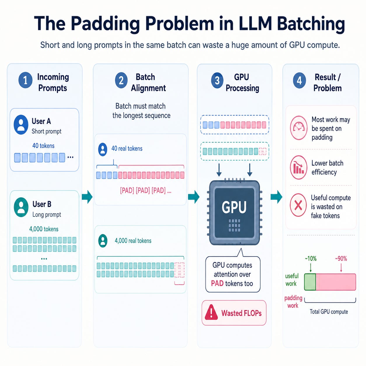
Let's start with the first problem: padding. Imagine you have two users, the first one sends you a prompt of forty tokens, and the second one sends you a prompt of four thousand tokens. To batch them together, you'll need to pad everything up to the longest sequence … and that's where the issue begins. The GPU doesn't know those [PAD] tokens are fake! It will happily burn real FLOPs computing attention over them (which, of course, is completely useless). In short, depending on the traffic mix you're dealing with, most of the compute in a batch can end up being work spent on ABSOLUTELY NOTHING.

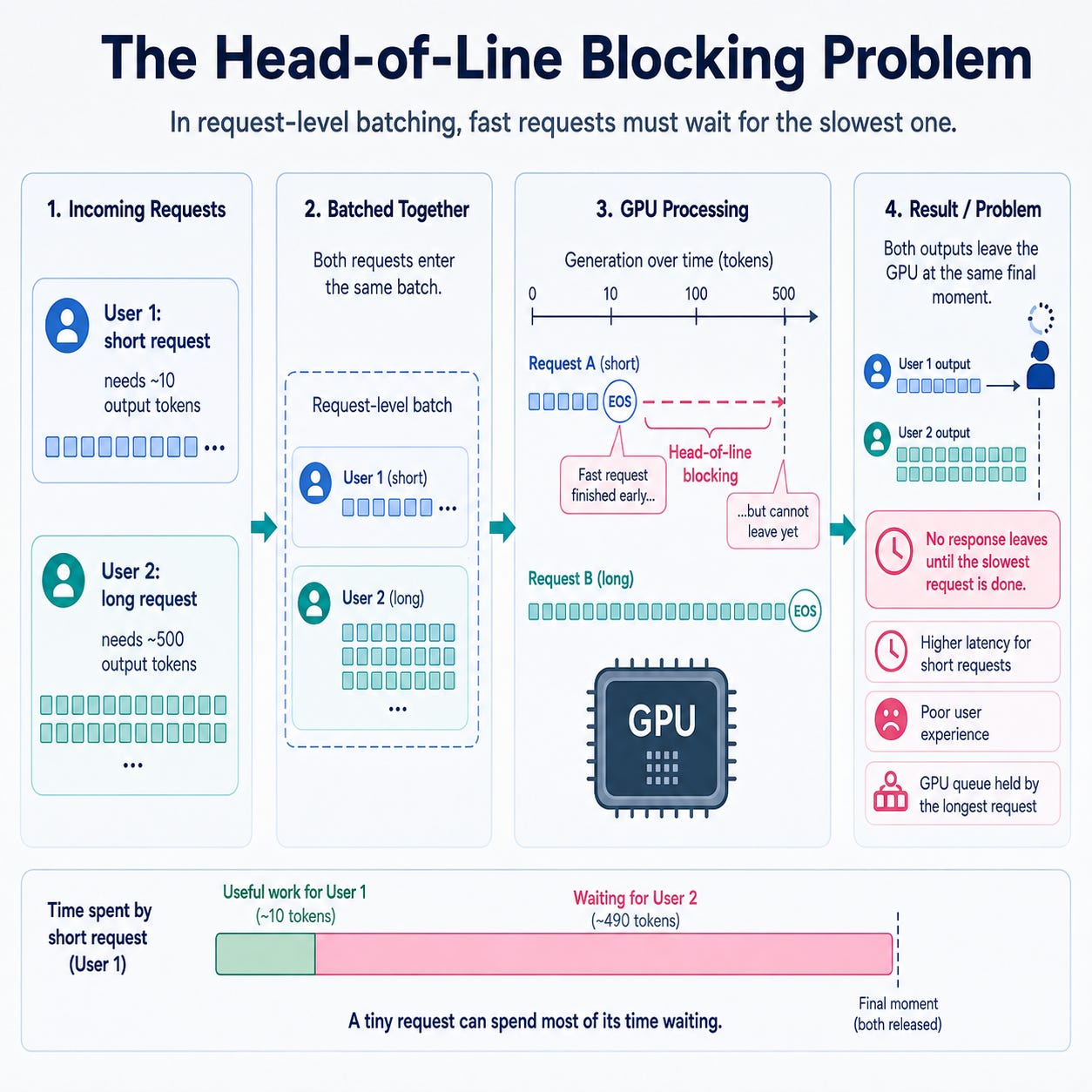
The second problem is even nastier, and it has a proper name too: head-of-line blocking. Let's reuse the same example as before: two users sending two different prompts of varying lengths. If request one finishes after ten tokens (it was just a 'Hi there' message) and request two needs five hundred tokens (like 'solve the relativity equations for me please'), request one just … sits there until request two is finished. In other words, with request-level batching, no requests leave the GPU until the slowest one is processed. Now, can you imagine the look on user 1's face, staring at a spinner waiting for a 'hi there' message to be replied to? Honestly, not ideal, and if I were the user, I would shut down that application for good.

The third problem concerns memory. Under "standard" PyTorch serving, every request gets a memory block allocated up front, whose size is designed for the worst case (remember, we should always be pessimistic when designing AI Systems!). But the problem is that, in the real world, generations almost never get anywhere near the reserved memory size. And what's the result? Well, between 60% and 80% of your VRAM is reserved for tokens that will never exist. And you are paying for the full A100 GPU, my friend.

The solution, which was first developed by Orca and then became well known because of vLLM, involves changing the level of detail: instead of scheduling batches of requests, individual iterations should be scheduled, that is to say single steps of token generation. Meet continuous batching.

In other words, following each forward pass, the scheduler examines all the active sequences. Once a sequence has just produced <eos>, it is immediately evicted and the associated memory is freed right away. Sequences that are waiting in the queue are then included in the running batch for the next iteration. Batch boundaries no longer exist since the batch never actually starts or finishes; it's a dynamic entity that sheds completed tasks and takes in new ones every few milliseconds, and the tensor cores never get a chance to idle.

Simple idea? Yes, it is. But it took the industry a surprisingly long time to arrive at it!

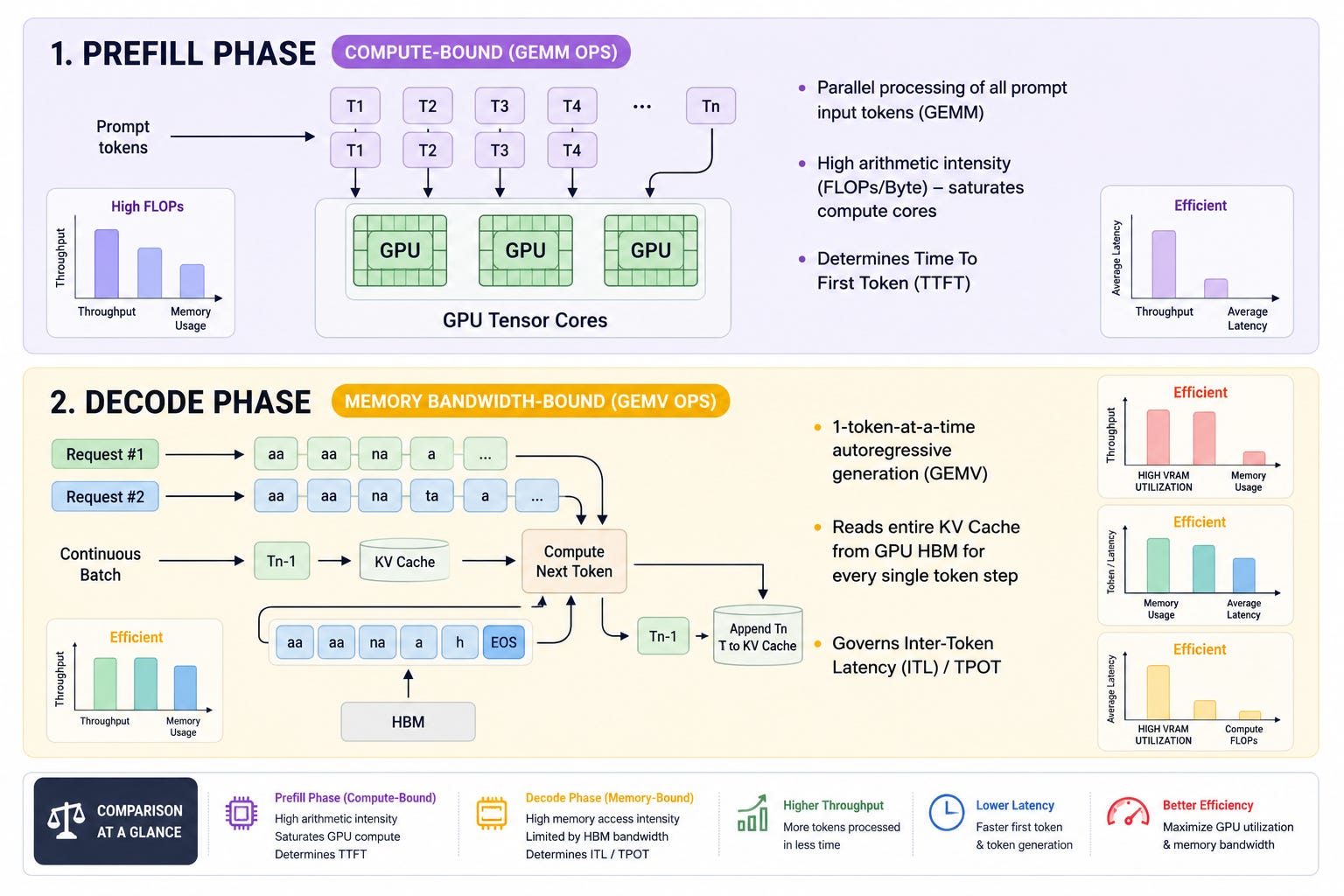
If you want to build inference pipelines that actually perform, there's one idea you need to internalize first: a single LLM request isn't one workload, it's two. And these two phases stress completely different parts of the GPU while being forced to share the same one.

During prefill, the model ingests your entire prompt, all N tokens of it, in one shot. Since every token is already there, nothing has to wait for anything else, so the whole thing collapses into big dense matrix multiplications (GEMM routines) that can saturate the CUDA cores and Tensor Cores.

• Arithmetic intensity: high (FLOPs per byte comfortably above 100). The GPU spends its time doing math instead of waiting around for memory transfers.

• Bottleneck: Tensor Core compute throughput (TFLOPs).

• What the user feels: Time To First Token (TTFT).

One caveat worth keeping in mind: this only holds for prompts long enough to fill the pipeline. A 12 token prompt saturates nothing, and behaves much more like the phase we're about to talk about.

Prefill ends and we drop into the autoregressive loop, one token at a time. To produce token t+1, the model needs the vector representation of token t plus the Key-Value cache of everything that came before it.

• Arithmetic intensity: terrible! (1 to 2 FLOPs per byte). For every single token you generate, the GPU has to drag all of the model weights out of High Bandwidth Memory (HBM) into SRAM, do a vector-matrix multiplication (GEMV), and write the updated KV state back to HBM.

• Bottleneck: GPU memory bandwidth (GB/s, or TB/s if you’re lucky).

• What the user feels: Inter-Token Latency (ITL), also called Time Per Output Token (TPOT).

If you want a feel for how brutal that is, do the back-of-the-envelope. A 14B model in FP16 is roughly 28 GB of weights. On an H100 with about 3.35 TB/s of bandwidth, you can move those weights around 120 times per second, and since you need one full pass per token, that's your ceiling: ~120 tokens/s for a single sequence, assuming perfect bandwidth utilization, which you will never get. The math doesn't care how many CUDA cores are sitting idle.

Which is also the answer to "why bother batching at all". Those weights get loaded whether you're serving one sequence or sixty-four, so every extra sequence in the batch rides along essentially for free. That's the whole game in decode: amortize the weight loading across as many sequences as you can fit.

To avoid recomputing the Key and Value projections for previous tokens on every single decode step, models cache those tensors in VRAM. For one request, the footprint looks like this:

Where:

• 2 is there because we store Keys and Values separately.

• N_layers​ is the number of transformer layers.

• N_kv-heads​ is the number of Key / Value heads, not query heads. This matters a lot, because Grouped-Query and Multi-Query Attention exist precisely to shrink this number.

• d_head​ is the dimension per head, which is the hidden size divided by the number of attention heads.

• L_seq​ is the full sequence length, prompt plus everything generated so far.

• bytes per element is 2 for FP16 / BF16, or 1 if you quantize the cache to FP8 or INT8.

Let's put numbers on it. Take Qwen 2.5 14B: 48 layers, 8 KV heads, head dimension of 128, running in FP16, at a 4096 token context.

Zero point seven five gigabytes for one single request. Now serve 32 of them concurrently and you're at 24 GB of VRAM doing nothing but remembering what has already been said. On an 80 GB card, that’s most of what you had left after the weights. And remember from the previous section that with naive allocation, the large majority of those 24 GB is reserved for tokens that will never be generated.

Before 2023, serving frameworks handled the KV cache the obvious way: one contiguous physical array in VRAM per request. And since you have no idea how long a generation is going to run, you allocate for the worst case, which means every incoming request immediately claims a slab big enough for Lmax=4096 tokens whether it ends up using 40 of them or all of them.

This wastes memory in three different ways, and it's worth separating them because they have different fixes:

• Reserved memory. Space that the request will eventually use, but isn't using yet. It's booked from token one and sits idle until the generation catches up to it.

• Internal fragmentation. The part of that slab that never gets touched at all, because the request finished at token 200 and you reserved for 4096. This is the big one, and it's pure loss.

• External fragmentation. Gaps between the slabs themselves. Requests come in with different max lengths, the allocator carves out differently sized chunks, and you end up with free space that's real but unusable because no single hole is big enough for the next arrival.

Put those together and you land where we left off in the last section: 60% to 80% of the GPU's memory doing nothing useful. Your concurrency ceiling ends up being a fraction of what the hardware could actually support, and you're not compute limited or bandwidth limited, you're limited by bookkeeping.

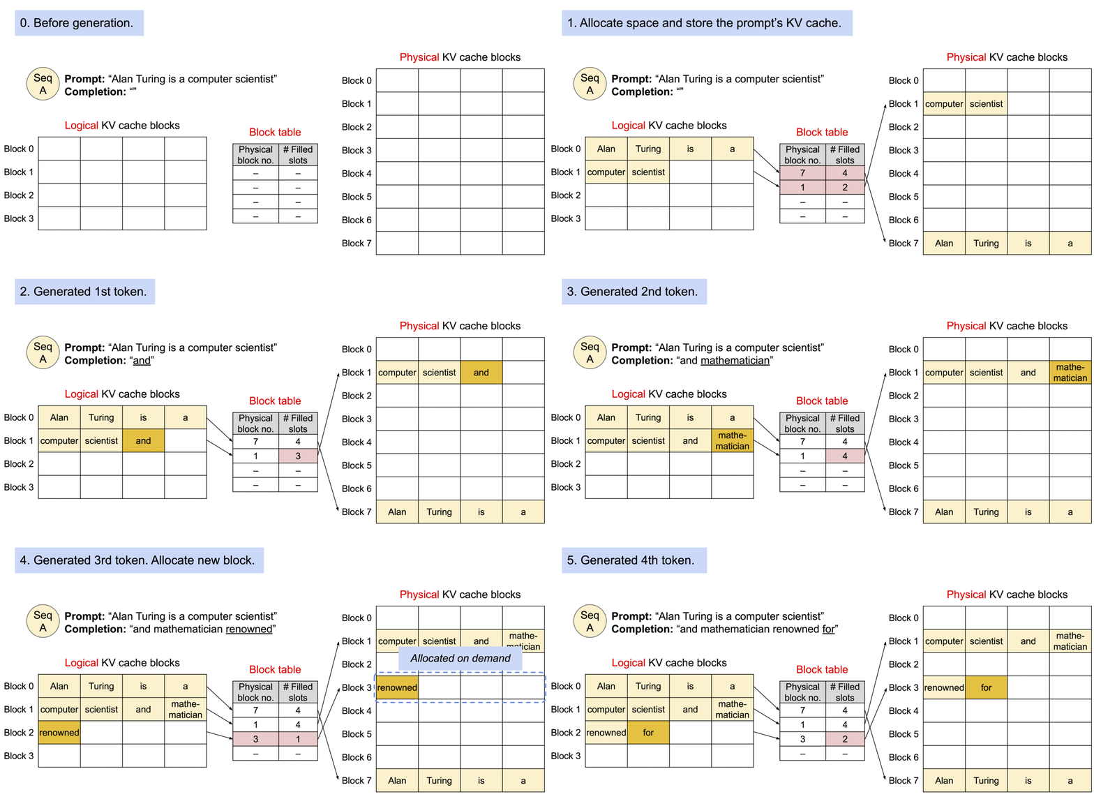
In September 2023, Kwon et al. published PagedAttention, which is the idea vLLM is built around. The insight is one of those things that feels obvious in hindsight: operating systems solved this exact problem decades ago with virtual memory paging, so stop demanding contiguous physical memory and start paging the KV cache instead.

PagedAttention chops the cache into fixed-size blocks, typically 16 tokens each (that's vLLM's default), and wires them together with three pieces:

1. Logical blocks. As far as the sequence is concerned, its KV cache is still one continuous stream of tokens, just divided into numbered blocks. Nothing about the model changes.

2. A physical block pool. The engine owns one central pool of same-sized VRAM blocks and hands them out on demand, one at a time, as sequences actually grow into them.

3. A block table. Each sequence keeps a small table mapping its logical block indices to wherever those blocks physically landed. The physical blocks can be scattered anywhere in VRAM, and the attention kernel is written to gather from them directly.

That last point is the part people gloss over. This isn't just a smarter allocator sitting on top of the usual attention implementation, it's a custom kernel that knows how to read Keys and Values from non-contiguous pages. You can't get here with a memory management trick alone. And now that we understand how PagedAttention works, the next question is: what do you actually get out of it? Well, here are three (BIG) benefits you'd get.

• Waste drops to almost nothing. Because all blocks are identical in size, external fragmentation disappears completely: any free block fits any request. Reserved waste disappears too, since you only allocate a block once the sequence is about to fill it. What's left is the tail end of the last partial block of each sequence, which the paper measures at under 4% of memory.

• Throughput goes up 2x to 4x on the same hardware, compared to the systems that were state of the art at the time. Worth being precise about what's happening here: you're not making the model faster, you're fitting far more sequences into the same VRAM, and as we saw in the decode section, extra sequences in the batch essentially ride along for free on weight loads you were already paying for. Bigger batches, better amortization, more tokens per second out the door.

• And the model output is bit-for-bit identical. No approximation, no quantization, no tradeoff to negotiate with your product team. Same math, better memory layout.

One bonus that pays off later: once your cache is paged, blocks become shareable. Two sequences with the same prompt prefix can point at the same physical blocks with a copy-on-write flag, which is what makes prefix caching and parallel sampling cheap. We'll come back to that.

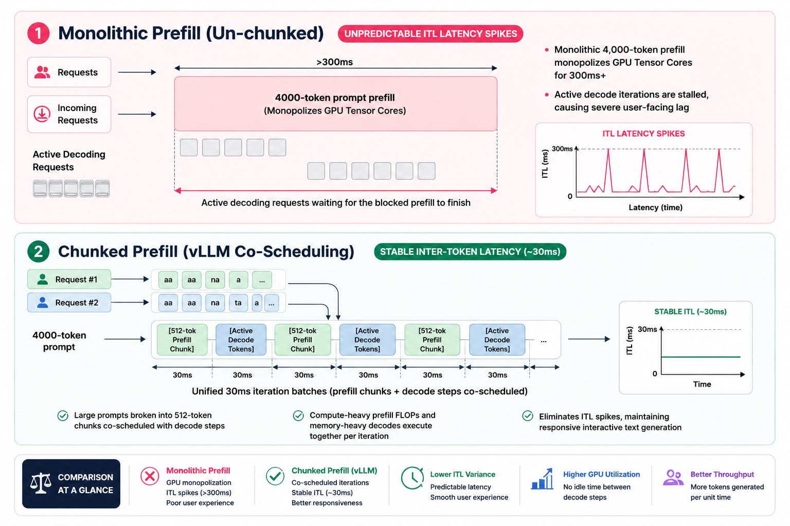
Continuous batching and PagedAttention fix the memory story, but they hand you a new one. Once prefill and decode are sharing the same engine, they start stepping on each other. The name for this is prefill-decode interference, and it's the thing that makes a system with great throughput numbers still feel bad to use.

Picture a batch that's happily decoding 16 requests. Each iteration takes something like 15ms, tokens are streaming out, everyone's content. Then a new user shows up with a 4,000 token prompt.

If your engine handles that prefill in one monolithic pass:

• The prefill GEMM takes over the Tensor Cores for 300ms or more, because it genuinely has thousands of times more work to do than a decode step.

• All 16 decoding requests sit idle for that entire window. They're not blocked on memory or waiting their turn in a queue, the GPU is simply busy.

• From the user's side, this shows up as an Inter-Token Latency spike. Text that was flowing at a steady clip just stops dead for a third of a second, then resumes. Your average ITL might look fine in the dashboard while the experience feels broken.

And notice this gets worse the more traffic you have, not better. Every new long prompt that arrives is another stall injected into everyone else's stream. The throughput graph stays happy. The p99 latency graph does not.

The fix, introduced as stall-free batching in the Sarathi-Serve paper and now standard in vLLM, is to stop treating prefill as an atomic unit of work. Chunked prefill splits a long prompt into fixed-size pieces and feeds them to the GPU a chunk at a time, alongside the decodes that are already running.

The scheduler works against a token budget per iteration, which is the max_num_batched_tokens knob (2048 is a reasonable default to start from). Each iteration it does roughly this:

1. Take the decode steps that are waiting, one token each. With 16 active sequences, that's 16 tokens.

2. Spend whatever budget is left on the next slice of a pending prefill. So 2048 minus 16, call it 2032 tokens of prompt.

3. Run one forward pass over the whole mixed batch.

A 4,000 token prompt now finishes in two or three iterations instead of one, and critically, nothing was stalled while it happened. The decodes kept advancing the entire time.

Here's why this is close to free. The prefill chunk needs the model weights pulled out of HBM anyway, and as we saw earlier, weight loading is the entire cost of a decode step. So the decode tokens ride along on transfers that were already being paid for. Prefill brings the FLOPs and saturates the Tensor Cores, decode brings almost none and just needs the bandwidth, and you end up using both halves of the GPU at once instead of alternating between starving one and the other.

Chunked prefill isn't a pure win, and it's worth being straight about where it costs you.

That long prompt's TTFT gets slightly worse. You've spread its prefill across several iterations and interleaved other work into them, so the user who sent the 4,000 token prompt waits marginally longer for their first token than they would have under the monolithic approach. What you bought with that is everyone else's ITL staying flat. It's a deliberate trade: you're taking latency away from the many and giving a little of it to the one.

Very small chunks stop being efficient. Two reasons. Small GEMMs don't fill the Tensor Cores well, so you lose the arithmetic intensity that made prefill fast to begin with. And each chunk's attention has to read the KV cache of every chunk before it, so the total memory traffic for a prefill grows as you cut it finer. Push the chunk size too low and you're paying real overhead for smoothness you may not need.

So max_num_batched_tokens is your dial between the two SLAs. Smaller values favour ITL and interactive feel, larger values favour TTFT and raw prefill speed. Which way you turn it depends entirely on whether you're serving a chat UI or a batch summarisation job, which is a theme we’ll keep running into.

Plenty of real workloads send the same tokens over and over. A fixed system prompt on every request. A few-shot template that never changes. A multi-turn conversation where turn five re-sends everything from turns one through four before it gets to the new question. In all of those cases the engine is recomputing prefill for tokens it has already seen, which is pure waste.

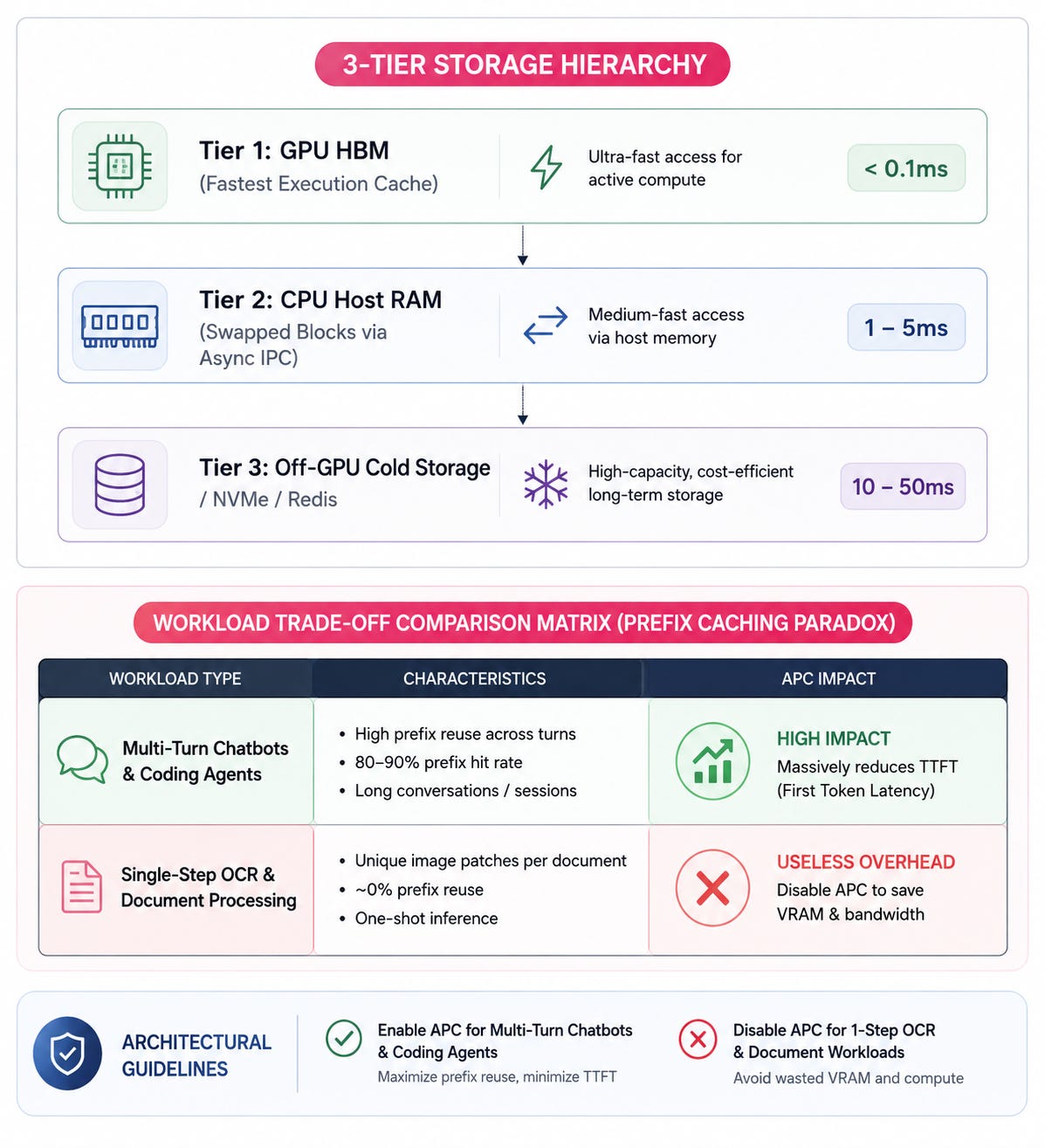
Automatic Prefix Caching (APC) kills that waste. Since PagedAttention already stores the KV cache in discrete blocks, and since a block’s contents are fully determined by the tokens in it plus everything before it, vLLM can hash each block and keep a lookup table of blocks it has already computed. A new request arrives, the engine hashes its prompt block by block, and every block that's already sitting in VRAM gets reused instead of recomputed.

That's the whole idea, and the payoff can be enormous. A request whose prompt is 90% cached prefix skips 90% of its prefill, which means TTFT drops by roughly the same amount and the Tensor Cores are freed for work that actually needs doing.

For large-scale enterprise deployments, KV cache management expands into a 3-tier storage architecture. In case you are interested, the diagram below showcases the tiers.

Now that we understand the basics of LLM Inference, and the optimization techniques behind engines like vLLM, let's translate theory into production infrastructure.

We'll deploy Baidu's Unlimited-OCR VLM pipeline as a high-performance asynchronous API on Azure Kubernetes Engine (AKS).