Allium Arithmetic for LLM Inference

A selection of cultivated alliums, at a Birmingham show.

Photo by Andy Mabbett, Creative Commons Share Alike 3.0
Birmingham was where I first worked on computers!

A microscaled set of 16 values and one scale facto can be considered vector in 16-space where the scale factor is the magnitude and the 16 values are coordinates giving the direction. This is not the usual way that microscaling has been used, but it has some properties that could make it interesting.

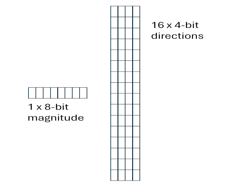
Since the precision is low it is fun to think of it as a fuzzball at the end of a stalk, somewhere in 16-dimensional space. An array of them would be a strange meadow!

When we do arithmetic with them at it looks just like other micro-scaled formats. An inner product (aka cosine) A·B just multiplies the magnitudes to get a new magnitude, then multiplies each of the 16 elements with its match on the other vector and adds them all to give the cosine factor. This multiplies the new magnitude to give a final result for this set of 16, and since these are normally just part of a much longer reduction these will then roll up along the reduction dimension.

Inner product can be optimized from the magnitude and interpretation of the directions.

The magnitude can be a pure exponent but with a fractional base. For example, it can be based on sqrt(2) which would give one fractional bit of precision. The microscale is a shared exponent. This allows simple addition for A.scale + B.scale.

The directions can amortize their adders in a tree which defers the carry logic by feeding carry into the next level of the tree. The whole tree benefits from sharing the scale. I plan to implement the RTL for this logic and estimate the energy it consumes. Some preliminary sketches show good efficiency.

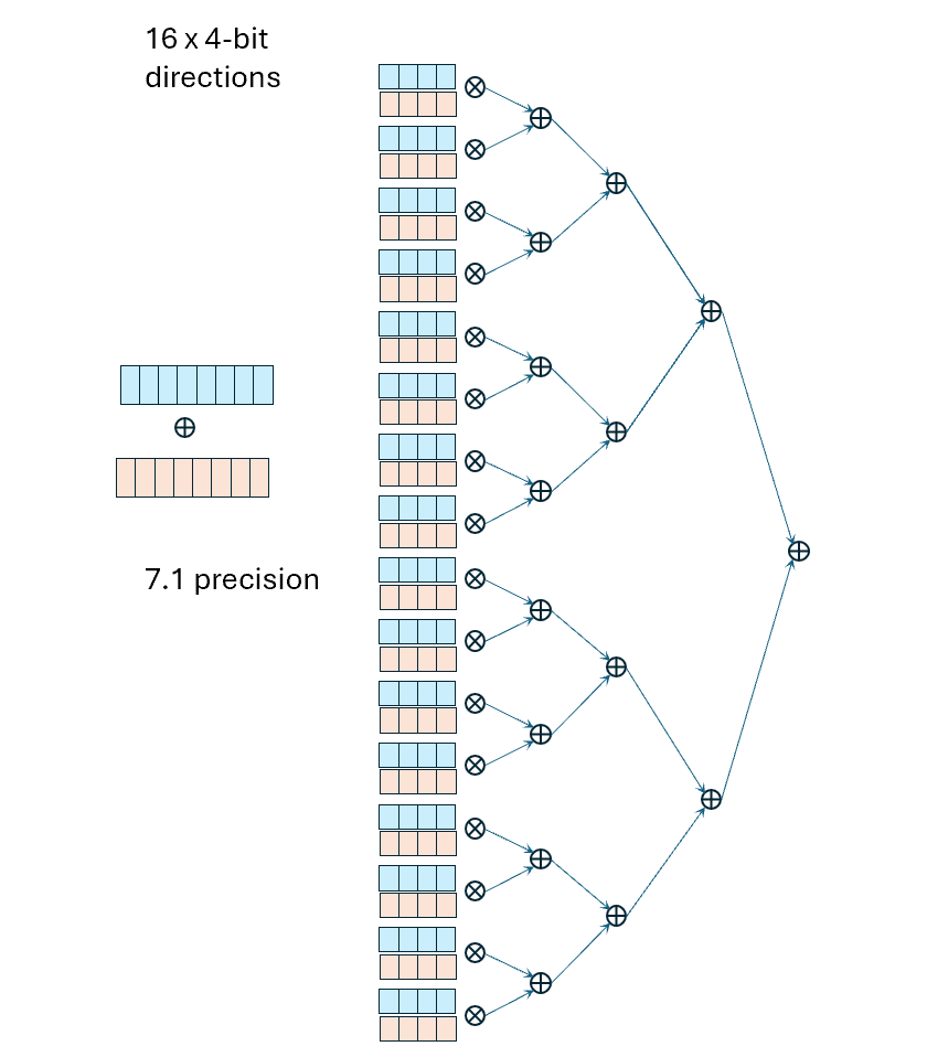
There are reasons to consider either FP4 and Int4 in the directions. FP4 is a bit like arc-tangent in making directions evenly spaced. However, there is also an argument for Int4 as simpler arithmetic with credible geometry and equally compatible with ordinary addition and multiplication for the inner product calculations.

The exponent is then paired with the tree-sum to make an FP number for the vector cosine sum and accumulated with all others in the row to complete the reduction.

While there are multiple tensors and other calculations in an LLM at inference, two things dominate the computational burden: self-attention, and the feed-forward-network (FFN, aka neural net or expert). These actually have closely related structure. Let’s begin with the attention.

I found it mysterious that one stream of input gets converted to Keys, Values, and Queries. Many texts will explain how the input tokens expand into embeddings which represent ideas. If you have not seen that then go read up on it.

But then these get transformed into 3 variants, why? The query retains the function of “what is usual context for this idea?”. The Key is a transformation of that same embedded idea but making a “recognizable idea”. Thus the first part of self attention is to run an inner product – a test of similarity – between “find related context” against every “recognizable idea” in the previous tokens. A single rating is generated for each context token for the level of interest, their relevance.

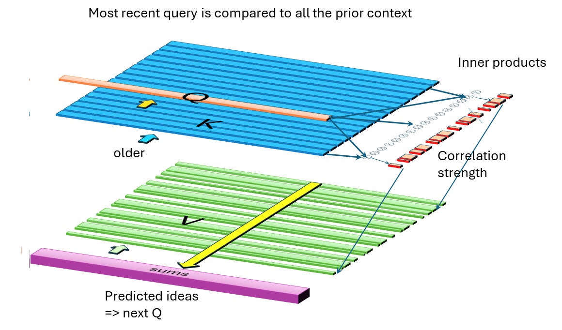
That leaves values, which are “what does this context tend to produce?” and we have one of those for every past token, so we multiply the relevance score times that value, and add all the relevance-values together. This becomes the sum of ideas about what comes next.

There are some important refinements, mostly normalization and sparsity.

Look at the correlation strengths. Some of these are large, some are small. Overall they tend to add up to a large number, because there are many rows in the context. However, we do not want a large number out. We are not creating an amplifier, we are searching for correlated ideas. Normalization starts by dividing the correlations so they tend to sum to a modest number, a typical predicted idea number.

This is done in a non-linear way often inspired by probability distributions but other functions can be used. Overall, what these tend to do is keep the best correlations, tone down the maybes, and zero out the irrelevant.

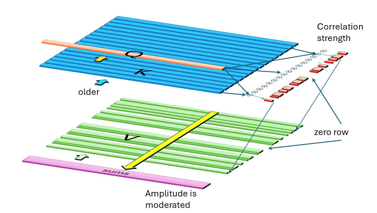
This sharpens the prediction but zeros can create sparsity in the V array, since any row with a zero correlation does not contribute to the sum. In fact you don’t even need to fetch that row from memory, if your hardware is nimble enough to modify the read requests in real time.

Another fun fact is that the correlations and sums can run in parallel and out of order.

The forward feedback network is a relative of a crossbar connection. It connects incoming ideas to refined outputs, with a flexible strength of connection. While neuromorphic computation does that using wiring and maybe programming some variable resistance and summation of the flow through crosspoints, the FFN or “expert” does this with arithmetic.

And, surprise, it is a very similar set of arithmetic to self-attention. While self-attention compares learned ideas to themselves in a structure designed to make connections across time and sequence, the FFN learns during training to connect suggested ideas from the attentions stage to refined ideas specialized to topics. These experts recognize the shape of nascent ideas from the attention stage and clarify them as sharpened suggestions,

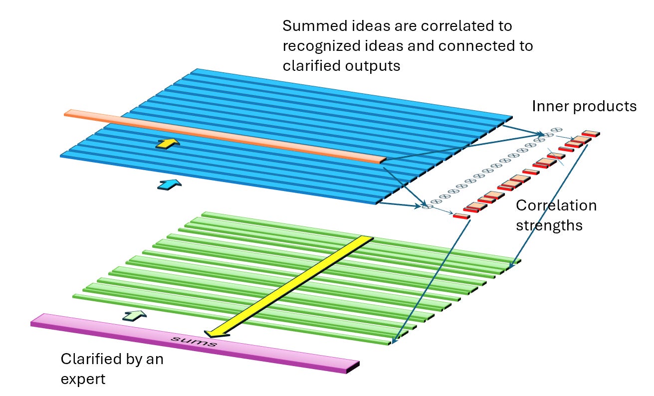
There is again normalization happening at the intermediate stage and potentially many of the output rows will have their correlation zeroed. The normalization functions used here do not need to be the same as in attention, and often they are not.

At this point though we have a very useful generic shape for the up-down correlation math.

Up to this point the heavy throughput has been the inner product for rows of the first tensor operation.

These inner products reduce to a correlation per row and those did do some fancy math for the normalization, but there were thousands of multiply-adds for each row reduction, so I gloss over normalization. Maybe a future topic.

The correlation needs to be applied back to the output row (in the V embeds or the Expert Down tensor). If the correlation is zero after normalization the entire row can be skipped. If non-zero it multiplies all the allium16 sets in the row, and that can be done by converting the correlation to an exponent which is added to the scales for each set.

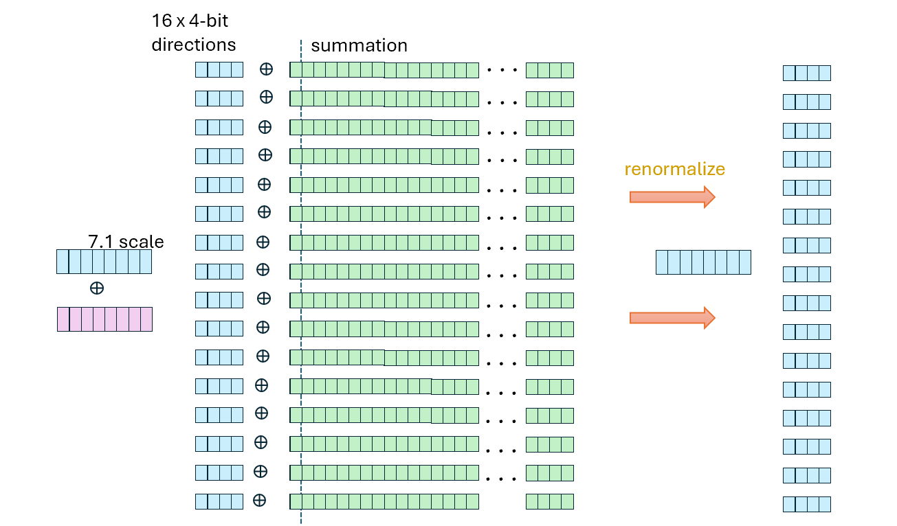
The normalization of the correlations can provide a maximum value of the result, which can be used to adjust the scale to line up with an integer summation. This multibit accumulator may look large but is less logic and energy than needed for FP32 or even BF16, since we can use minimal carry-look-ahead and just include incomplete carries in next round of summation. It results in extra cycles to finish but we are in a pipeline with hundreds of cycles already, a few extras are acceptable if they benefit us on power and size.

To recap, allium16 can be elements in reduction and summation to handle the two largest operations in inference, the up/down tensor pairs found in self-attention and in expert FFN.

Allium16 gives a concept to understand microscaled sets not merely as a quantization but as a different kind of number, a vector in 16-space, and that gives clarity on how to simplify the arithmetic.

We can combine the operators for inner product into a 16-wide fused multiply-add, and we can design the output summations to use a prescaled integer accumulator. Both of these are expected to have good energy per operation and to fit in a reasonable area of the silicon.

In future weeks I plan to:

• Use EDA tools to obtain the PPA for both

• Compare the results in actual LLM data and weights to see how they compare on accuracy

  Share

However, that work will take a while. The next article I plan to return to ECC and look at how much delay would occur if PCIe Gen7 would use a fix-any-4-symbol form of Reed Solomon code instead of 3 interleaved fix-1, and what the benefit could be.

Why bother?

Leave a comment

• The geometrical intuition and considering the entire set of 16 as one new kind of number helps think through how arithmetic units can be unified and optimized. It may also help in understanding how information maps into the numbers.

Will algorithm change make this obsolete?

• Maybe. But the up / down tensor pair is found in many places and tensors have been around for a long time. The allium16 approach seems likely to remain useful as it is easy to use and this will be reinforced if the arithmetic is efficient.

What happened to big systolic arrays? This looks like a vector processor.

• Correct. In inference the arithmetic intensity is very low for the KV Cache and for the weights in the experts, so while you could describe the data flow as systolic, rows arrive in pulses as fast as an HBM can deliver, the arithmetic is mostly vector since there is just one token per layer of the LLM and that token embedding is wider than the whole HBM interface of a GPU. So a vector is all you need. Even if the arrays are preloaded into SRAM the wide interface would only stack a few rows of a third dimension for a true tensor before reaching the practical throughput limit. So, studying this in wide-vector form is reasonable even for the highest performance in inference decode. Training and prefill may require more attention to the third dimension but I still expect the allium16 arithmetic to be useful and efficient.